
I’ve been wanting to do this for a while. In my undergraduate motion planning course, we learned how to make a point robot navigate a map using several motion planning algorithms — you may have encountered A*, PRM, RRT, and so on. However, when I first started working on problems with robot arms (or manipulators), I felt there was a lot missing to go from these simple 2D navigation examples to more complex manipulators.
At the time of writing, I count 7 years since I found myself in this situation. Since then, I’ve done a lot of learning, trying, messing up, and correcting. I’ve written blogs and videos for MATLAB and Simulink [1][2][3], created videos for RoboCup@Home Education, developed an academic service robot software stack, became a MoveIt maintainer, and recently created PyRoboPlan, an educational toolbox for robot manipulation written in Python. While my main focus in robotics remains high-level behavior and task planning, I would say motion planning for manipulators is a close second.
This post is… very long, but even so it’s my best attempt to distill my efforts so far. There are others who are more qualified to write this, but few of them will consider it and even fewer will actually do it, so here we are. I will talk about what it takes to model a robot manipulator, the main algorithmic components you may encounter (including their well-known and state-of-the-art implementations), and the software tools you should know if you choose to build your own motion planning stack. Enjoy the ride!
Table of Contents
The Motion Planning Landscape
So… what is motion planning? I usually begin my answer with a wildly reductive definition: moving from point A to point B without doing bad things.
Let’s expand on these:
- Moving from point A to point B: Normally, “point A” refers to the current state of the robot, but that’s not necessarily true; you could be planning for a future hypothetical state. “Point B” often denotes a target configuration (joint positions, velocities, forces, torques, etc.) or pose (Cartesian position and/or orientation of a particular location on the robot, and similar derived quantities). This could also be a list of targets, such as a reference tool path to follow — think, for example, of a robot trying to draw a multi-segment line on a whiteboard.
- Doing bad things: The most obvious “bad thing” is not hitting stuff, which could be self-collisions or contact with the environment. The astute reader may notice this implies we know what both the robot and environment look like to a collision checker, which we’ll get to later. There are other safety-related considerations, like staying within joint limits (position, velocity, acceleration, torque, etc.). Finally, there may be constraints not related to safety, but rather to user preferences. To name a few examples, a motion planning problem may be imbued with position or orientation constraints (for example, moving a water cup without spilling it), or biases to keep the robot as close as possible to a specific nominal joint state to avoid inefficient motions (like getting close to areas that are unsafe or have poor maneuverability, or requiring too much motor current).
The technical jargon for achieving this magical conversion of goals to low-level actuator commands that move the robot safely can be summarized with the following diagram.
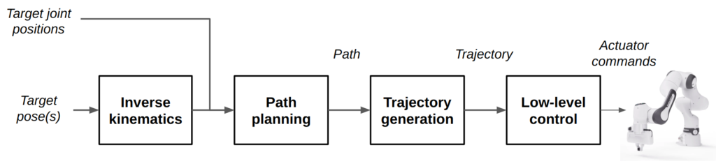
Before going any further, it is important to understand the distinction between a path and a trajectory.
- Paths generally describe a sequence of joint positions (or Cartesian poses) that solve our “point A to point B” problem. They could be as simple as a straight line from A to B, or contain a list of dozens of waypoints needed to navigate an obstacle-ridden environment.
- Trajectories, on the other hand, augment paths with timing information. They are usually mathematical expressions that can be evaluated to describe positions, velocities, accelerations, etc. as a function of time. These functions then get evaluated by a low-level controller, which seeks to track the trajectories over time.
While the later sections get into more detail, I will briefly explain the individual components in the diagram:
- Inverse kinematics: Solving for valid joint positions that achieve a specific Cartesian pose for a specific frame on the robot. This is in contrast to the significantly easier forward kinematics, which is doing geometry (or as Professor Francis Moon called it in my intro class, “high school math”) to calculate this pose given a set of joint angles.
- Path planning: Finding a list of joint positions and/or poses that actually move the robot from a start to a goal configuration. This could also take into account any constraints (collisions, joint limits, etc.) in our planning problem.
- Trajectory generation: Converting a path to a time-based trajectory for execution by a low-level controller. While trajectory generation classically has been used to “time-parameterize” a path output by a planner, it is also common for path planning and trajectory generation to be done jointly. For example, trajectory optimization methods can directly return a trajectory that achieves a reference pose under our aforementioned constraints. Plus, it can include new constraints introduced by the time aspect, such as maximum velocities, accelerations, torques, etc.
- Low-level control: The software that accepts a trajectory and applies control techniques (such as PID, MPC, etc.) so the robot’s actuators follow the trajectory. We won’t talk about this component very much here, so if you’re interested in controls, this is almost all you will get.
Notice, by the way, that nothing in this section was unique to manipulators. While this holds true for most of this post, there will be some bias towards tools and approaches applied in systems with more degrees of freedom, such as manipulators and legged robots.
Modeling Your Robot Arm
Before we go into the core components of motion planning, we should cover some of the foundations. This includes how to mathematically represent robot manipulators to facilitate motion planning, as well as some key concepts and software representations that will help you better digest the later sections.
Rigid-Body Mechanics
When dealing with manipulators, we often start with a massive simplifying assumption that they are made up of rigid bodies. This works in most cases, but I (and no doubt many others) would be unhappy if I didn’t mention the entire field of soft robotics. While many techniques in this post can be applied to compliant systems, you do need more sophisticated models and assumptions to pull that off. By the way, even with “rigid” metal robots you might need to consider vibrations and/or bending under particularly strenuous or high-precision conditions. So yeah, all models are wrong, but some are useful.
With the rigid body assumption, we can say that our robot is made up of rigid links and joints that define motion between them. Joints can be either revolute (rotational motion) or prismatic (translational motion). Although software tools can have other types of joint representations, either for convenience or to deal with numerical issues, all joints are derived from combinations of these two basic ones.
With this information, we can now perform forward kinematics (FK). This uses the (static) transforms between links, and the joint positions, often referred to as the configuration, to compute the (dynamic) transforms between moving coordinate frames. By far, the most common application of FK for manipulators is to find the pose of the end effector (gripper, hand, etc.) with respect to the robot base or world, given a set of joint positions.
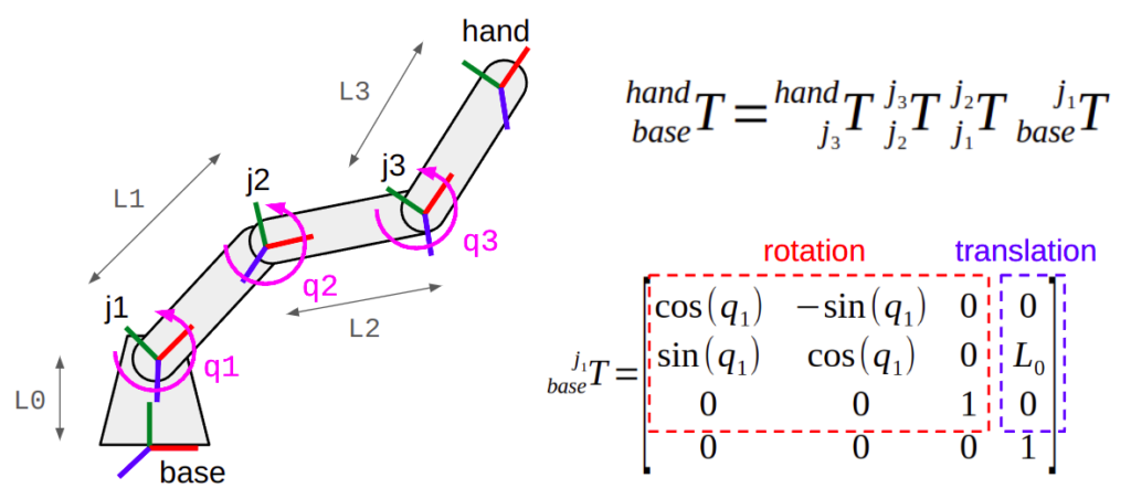
(Top Right) The transform between two coordinate frames can be expressed as a composition of transformations along a kinematic chain.
(Bottom Right) Some transforms are dependent on the joint positions (angles for revolute joints, translations for prismatic joints).
Degrees of Freedom, Actuation, and Redundancy
Roughly speaking, the number of independent dimensions that a robot can move in defines its degrees of freedom (DOF). For example, a manipulator with 3 joints has 3 degrees of freedom. There may be additional constraints that reduce this number; for example, four-bar linkage or slider-crank mechanisms effectively turn four joints into a single degree of freedom due to mechanical coupling. To learn more, check out this video from Kevin Lynch and Frank Park’s Modern Robotics textbook, which will be cited in many other places here.
It is also important to note that a robot doesn’t necessarily have direct control of all its degrees of freedom. As such, there are 3 categories of robots by their ratio of actuators to degrees of freedom.
- Fully actuated: Has exactly one actuator per degree of freedom. In practice, most robot manipulators are fully actuated because they need to stay upright without moving, but also require precise control in every dimension to manipulate objects.
- Underactuated: Has less actuators than degrees of freedom. These designs are often seen in dynamic systems like legged robots; for example, with passive ankles that have springs (sometimes actual springs, sometimes compliant surfaces) instead of actuators.
- Overactuated: Has more actuators than degrees of freedom. One example is a multi-rotor aircraft with more than 6 motors and propellers. The additional actuators are not necessary for 6-DOF control, but can be useful in case one or more propellers break, or maybe because the extra thrust is needed to keep the vehicle mass airborne with the chosen actuator sizing. You can also put multiple actuators on a single joint in articulated systems like manipulators or legged robots, but it requires very good controls to not make the actuators end up “fighting” each other… so its not common.
There is one more consideration with manipulators. The only way that an end effector can be positioned in any valid reachable pose with at least 6 well-designed* degrees of freedom; 3 translation and 3 rotation. If a manipulator has more than 6 DOF, it is referred to as a redundant manipulator. We will get back to this later, but redundancy can be extremely useful when planning needs to take into account constraints such as collision avoidance, joint limits, or even user preferences for what motion should look like. If you want to go deeper into this topic, the article “How many axes does my robot need?” is a good starting resource.
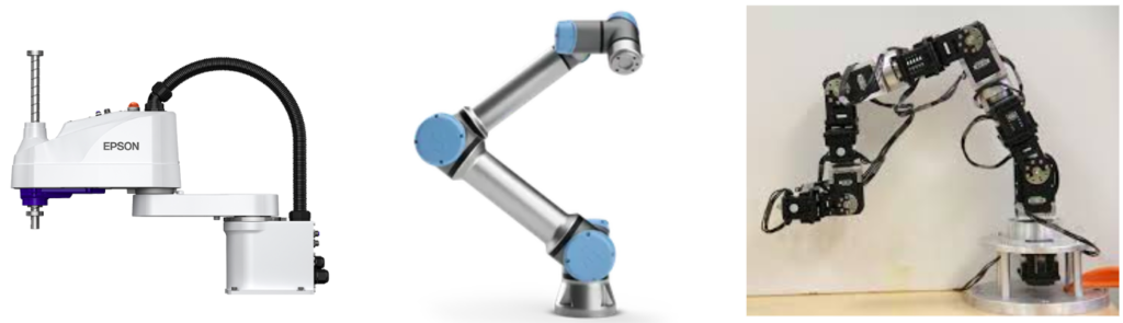
(Middle) Universal Robots UR5e has exactly 6 DOF.
(Right) Experimental 9-DOF redundant arm from a Master’s Thesis at the University of Dayton. I highly recommend watching this video.
* I say 6 well-designed degrees of freedom, because you could for example have a robot with 6 joints that only allow motion on a single plane. Here, the end effector can only be controlled along 3 independent dimensions. Is this considered a redundant arm, then?
Who’s this Jacobi guy, anyway?
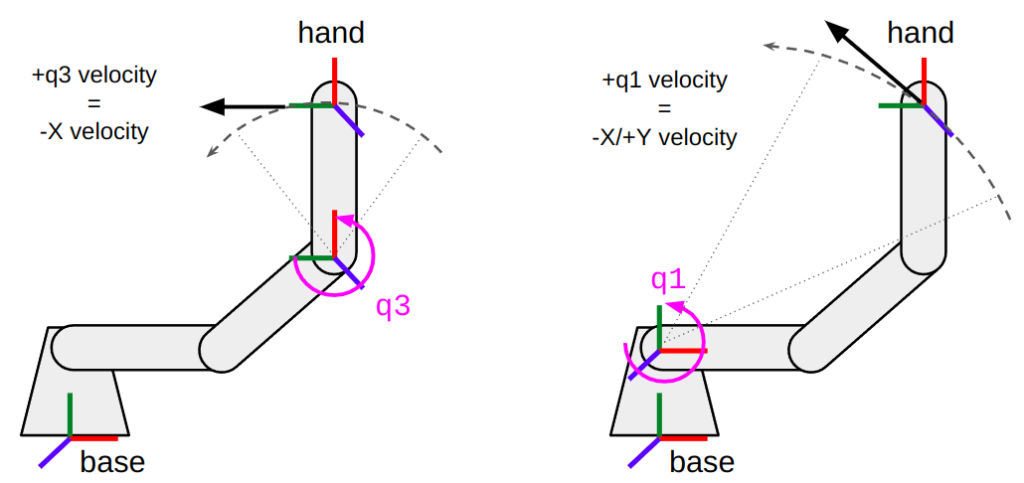
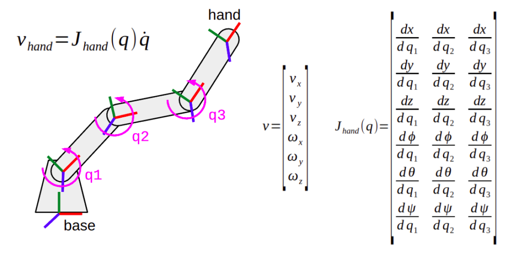
Here’s a thought experiment. Suppose you want to know the effects of moving a joint on the position of a specific frame on your robot, such as the end effector. Just like with forward kinematics, this calculation depends on the current joint configuration of the robot. Take a look at the image below.
- On the left, you see that rotating the third joint with a positive velocity will cause the hand to move along an arc whose tangent at that particular position happens to be along the -X direction in the base frame (or +Y in the hand frame).
- On the right, you see that moving the first joint instead will cause local motion along both the -X and +Y directions in the base frame. Because this arc has a bigger radius, as the joint is farther away from the hand, this joint motion also has a greater effect.
In both cases, the hand frame will also rotate about the +Z direction. You can imagine how this becomes more complex with a robot that doesn’t exist purely on a 2D plane.
hand frame to move along the -X direction in the base frame.(Right) At the same configuration, rotational motion about the first joint causes the
hand frame to move in a different direction. Because this joint is farther away from the frame, it also has a larger effect compared to closer joints.The general way to express these relationships is through a matrix named the geometric Jacobian. Jacobians are critical in several applications within robot motion planning and control. This includes inverse kinematics, teleoperation (or servoing), low-level position and force control, and even enforcing task space and collision constraints within path planning and trajectory generation. This is why I am writing so much about them, and why it won’t be the last time they come up in this post.
If you have a background in mathematics (or have access to Wikipedia), you may know Jacobians as defining the gradients of some function with respect to its variables, and packaging that up into a neat matrix. In the context of robot manipulators, the geometric Jacobian uses the first derivatives of the robot kinematics to tell you the relationship between the joint velocities and the six Cartesian (or task space) velocities — that is, XYZ translational and rotational velocity. To get into more detail, you should watch this video.
NOTE 1: The geometric Jacobian also applies to the derivatives of velocity, like acceleration, jerk, snap, crackle, pop, etc… but not positions! This is why the reverse problem of calculating joint positions from Cartesian pose, or inverse kinematics, has its own section.
NOTE 2: The qualifier “geometric” is used in this case, because there are other types of Jacobians that will similarly associate joint torques and task space generalized forces (forces and torques about XYZ) using not the kinematics, but the dynamics of the robot. The math is similar, but instead of lengths and angles we’re now dealing with mass, inertia, stiffness, damping, and all that good stuff we’ve been ignoring so far.
What is interesting is that Jacobian matrices are not necessarily square — they only are if the robot has exactly 6 degrees of freedom. Even in the case of a 6-DOF system, it’s not necessary that the Jacobian at a particular configuration has full manipulability in all directions (in math terms, the matrix is not full rank); our “6 joints on a single plane” example from the previous section is one such case. This means that you often can’t “just invert” the Jacobian to go the other way and get joint velocities out of task space velocities. We’ll explore the ramifications of this in a later section.
Collision Checking
Our rigid-body models so far don’t capture whether a specific joint configuration or path is free of self-collisions or collisions with the environment. Usually, we need to augment these models with additional geometric information that can be used to check collisions.
Most modern collision checking libraries, such as Flexible Collision Library (FCL), can be used to perform these computations. Collision geometries can be represented as simple primitives (spheres, cylinders, boxes, etc.) or as meshes that can directly come from CAD models. This presents a tradeoff: while collisions between geometric primitives are relatively inexpensive to compute compared to meshes, they are approximations of the true geometry of a robot. Often, robot modeling frameworks have a distinction between the visual geometry (full-resolution meshes to visualize the robot) and collision geometry (a combination of simple primitives and coarse collision meshes). If you want to learn more, I would recommend looking at the official FCL paper, published at ICRA 2012.
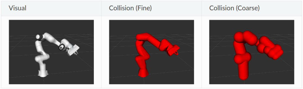
Source: franka_ros documentation
We also need to talk about collision checking with the environment. It is true that we can also use geometric primitives and meshes to represent the world around the robot. This works if we know what the environment looks like a priori (for example, the robot is in an industrial workcell) or we have a mechanism to detect objects and fit shapes (like boxes) around them. However, you can also directly use sensor data to treat the whole environment as an obstacle. One common approach is to convert point clouds from depth cameras and/or lidar into representations amenable to collision checking. A format supported in many software libraries is Octomap, which is just a more efficient way of representing a voxel grid in software.
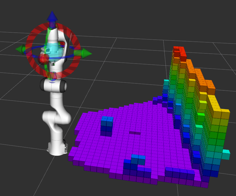
Source: MoveIt documentation.
Notice, by the way, that some geometries in our models may always collide with each other. This is sometimes expected for adjacent geometries on the same link, or directly across a joint boundary, but less so for more distant geometries. Most modeling frameworks let you define a list of collision pairs to be checked, instead of exhaustively checking every possible pair. Moreover, this list of pairs can often change on the fly. For example, if your robot is closing its gripper fingers around an object, maybe it’s okay that the model ignores the collision between the fingers and the object… but if you were planning to move somewhere else, you don’t want to end up knocking the object with the back of the fingers.
Another related representation used in motion planning, which is also common in computer graphics and game development, is the signed distance function or signed distance field (either way, it abbreviates to SDF). SDFs, as their name suggests, return a distance value that is positive if geometries are not in collision, and negative if they are in collision, zero being right at the edge. These can be analytical functions for simple primitives, but it is also common practice to generate SDFs offline from more complex shapes (meshes, Octomaps, etc.) and store them in memory for quick lookup at runtime. For a basic introduction to SDFs, I like this YouTube explainer. Closer to our robotics applications, you will find that state-of-the-art software tools like MuJoCo and nvblox have support for SDFs.
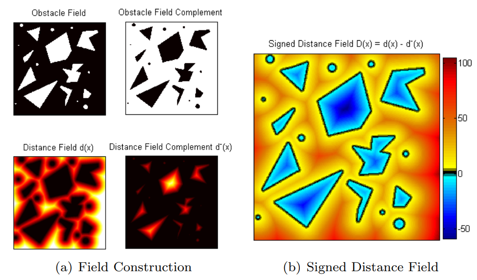
Source: Zucker et al. (2012)
Robot Description File Formats
Ultimately, our robot model representation needs to work with various types of software, including simulators, motion planning frameworks, control tools, etc. While there is no “one format to rule them all”, there have been several attempts to standardize. In my opinion, these are the surviving ones at the time of writing:
- Universal Scene Description (USD), developed by Pixar, is the de facto scene representation format in the computer graphics and 3D animation community.
- SDFormat (Simulation Description Format, confusingly also abbreviated to SDF) is an XML based format that was first developed for, and still used by, the Gazebo simulator.
- Also coming out of the ROS ecosystem and XML based is Universal Robotic Description Format (URDF). I don’t think it’s controversial to say this is the de facto standard for rigid-body robot descriptions. Most robotics software tools support URDF import, most CAD software tools like SolidWorks, Onshape, etc. have a URDF exporter, and there are even USD to URDF converters.
To learn more about URDF, refer to the official tutorials; or if you prefer videos, I recommend the Articulated Robotics YouTube channel. In fact, Articulated Robotics has such good content that I am directly embedding the video here.
XML based representations do not stop here. Specific to motion planning, you will also sometimes encounter a supplemental Semantic Robot Description Format (SRDF), which was pioneered by MoveIt, but is also used in other frameworks. This defines additional information that the URDF specification does not contain, including joint groups, saved joint configurations, and deactivated collision pairs. Below is a minimal example of an SRDF file, but that you can find more realistic ones in actual robot description packages.
<?xml version="1.0" encoding="UTF-8"?>
<robot name="my_robot">
    <!-- Joint groups -->
    <group name="arm">
        <joint name="arm_joint1"/>
        <joint name="arm_joint2"/>
        <joint name="arm_joint3"/>
    </group>
    <group name="hand">
        <joint name="finger_joint1"/>
        <joint name="finger_joint2"/>
    </group>
    <group name="arm_and_hand">
        <group name="arm"/>
        <group name="hand"/>
    </group>

    <!-- Saved states -->
    <group_state name="home" group="arm_and_hand">
        <joint name="finger_joint1" value="0.001"/>
        <joint name="arm_joint1" value="0"/>
        <joint name="arm_joint2" value="-0.785398"/>
        <joint name="arm_joint3" value="0"/>
    </group_state>

    <!-- Collision filters -->
    <disable_collisions link1="base_link" link2="shoulder_link" reason="Adjacent"/>
    <disable_collisions link1="shoulder_link" link2="elbow_link" reason="Adjacent"/>
    <disable_collisions link1="hand" link2="base_link" reason="Never"/>
</robot>
Motion Planning Components Explained
Now that we know how to model our manipulator, let’s return to actual motion planning. Strap yourself in for a deep dive into inverse kinematics, path planning, and trajectory generation. This section is where you will be exposed to well-established and state-of-the-art algorithms alike, as well as my personal insights into how these fit into our field’s existing toolkit for motion planning.
Inverse Kinematics
It is not natural for us to express the goals of a robot arm in joint positions. We often prefer to move a specific coordinate frame on the robot to a target pose (position and rotation). For example, this could be to place a robot hand on a door handle. This applies not only to single goals, but also for tasks that require following a tool path, such as welding, wiping a table, or pouring a cup. In all these situations, inverse kinematics (IK) is needed to convert these Cartesian goals in task space to their corresponding joint positions.
In an earlier section, I may have scared you into thinking that IK is impossibly hard. While it is harder than FK, there is a subset of problems in which IK can be solved analytically. If you can afford to do this, you absolutely should, as it makes the results consistent and the software implementation blazing fast. This is why several industrial arms have exactly 6 degrees of freedom and are designed with a spherical wrist mechanism that makes the math easier by decoupling IK into using the 3 wrist joints to solve for rotation and the other 3 to solve for position. While this math can be derived by hand, software tools exist to automatically generate analytical IK code from a robot description file, such as IKFast.
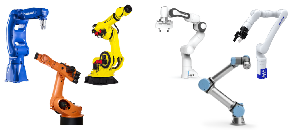
(Right) Collaborative robot (cobot) arms: Franka Research 3 (7-DOF), Universal Robots UR5e (6-DOF but no spherical wrist), and Kinova Gen3 (7-DOF).
In other cases, you may need to rely on numerical methods to solve IK. This isn’t always bad; while a redundant robot may have multiple (or even infinite) IK solutions for a given target pose, this redundancy can help produce solutions that satisfy additional constraints, like collision avoidance or position/orientation bounds. This is why most collaborative robot (cobot) arms like the ones in the diagram above rely on numerical IK solvers.
One simple numerical method that, in my experience, is rarely used, is Cyclic Coordinate Descent (CCD). By far the more common one is the Inverse Jacobian, or differential IK method, which I consider more mathematically principled and more extensible. We covered the geometric Jacobian earlier in this post, and here is one place where it surfaces. Roughly, what this method involves is the following calculations in a loop:
- Compute the pose error between the current and desired pose.
(Notice that getting the current pose requires forward kinematics!) - If the error is within some specified tolerance and meets any additional constraints, return the solution.
- Use the inverse Jacobian* to get a first-order approximation of joint velocities towards the desired pose.
- Take a step in that velocity direction.
* We say converting task space error to joint velocity requires inverting the Jacobian, but we established that this was not possible in the majority of cases. As such, we end up relying on the Moore-Penrose pseudoinverse, used in least-squares regression, or its close cousin damped least squares (or Levenberg-Marquardt) to deal with numerical instabilities (Don’t you miss the days where everyone stuck their names on every scrap of math they could find?). Some good resources to learn more are these slides by Stefan Schaal and this survey paper by Samuel Buss.
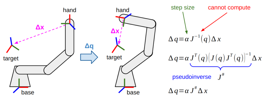
(Left) Visual representation of the pose error being reduced in a single optimization step.
(Right) The basic underlying equations. Since the geometric Jacobian relates Cartesian velocity with joint velocity, it can be (pseudo-)inverted to minimize pose error towards an IK solution.
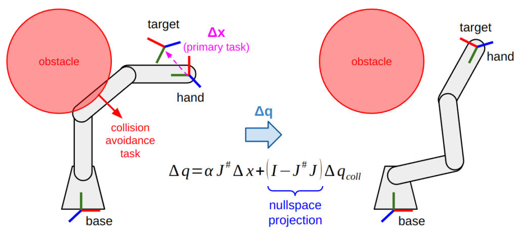
With a redundant manipulator, you can use these Jacobian based IK methods to solve for a primary task and a set of secondary tasks, so long as they don’t interfere with the primary task. This can be done by “zeroing out” all the components of the secondary task that would interfere with the primary task. Mathematically, this is done through nullspace projection. You can dive into the math around Equation (7) of Samuel Buss’ paper, or by watching this great video by Leopoldo Armesto.
This approach, by the way, is sometimes referred to as “stack of tasks” (SoT); one expert in this space is Stéphane Caron, who not only wrote a great blog post on IK, but also implemented a cool SoT based IK solver named Pink. The examples in the Pink repo demonstrate how far you can go with stacking tasks when working with high degree-of-freedom systems such as humanoid robots. Another good example is the Saturation in the Null Space (SNS) work by Fabrizio Flacco et al.
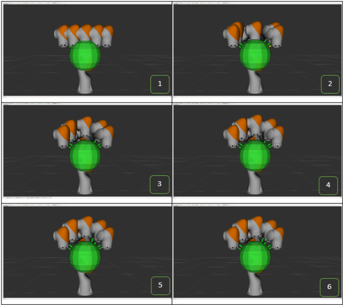
One example of stacking tasks is solving IK while avoiding collisions. If you have a redundant manipulator, maybe you can achieve your IK goal either with an “elbow up” or “elbow down” configuration. However, in this case the “elbow up” solution might be in collision. By adding a collision avoidance task and projecting it to the nullspace of the IK task, you can guide the solution towards the “elbow down” solution. This can also extend to constraints that push away from joint limits or towards joint specific positions, or keeping within position or orientation constraints in task space.
Another approach to solve IK is nonlinear optimization, which many state-of-the-art IK solvers apply. Some examples include:
- Saturation in the Null Space (SNS) methods, which use inverse Jacobian methods with nullspace projection in the basic algorithm, but then move on to use Quadratic Programming (QP) in their “Opt-SNS” variants. I highly recommend looking at the 2015 paper by Flacco et al. to see how this approach evolved.
- Drake’s suite of IK solvers, which all set up nonlinear optimization programs of some variety, as that is a key strength of Drake.
- TRAC-IK, which runs a regular inverse Jacobian IK solver (the KDL solver, to be precise) in parallel with a nonlinear optimization solver. It then returns the first solution it gets, or the “best” one within a given time budget (up to the user).
Indeed, both Drake and TRAC-IK rely on nonlinear optimization solver packages such as NLOpt and SNOPT, which support Sequential Quadratic Programming (SQP), to perform these optimizations with highly nonlinear manipulator kinematics and constraints.
Finally, it is worth mentioning that numerical methods are susceptible to local minima based on the initial conditions provided. While global optimization techniques have been applied to IK, these methods have their own drawbacks and have not yet become popular. For example, BioIK uses genetic algorithms, which can find global minima, but are also extremely computationally inefficient.
A lighter-weight, and shockingly effective, alternative is to add “random restarts” to solvers in hope that trying different initial conditions increases the likelihood of success. I can personally vouch for this; in a recent project, I was benchmarking an IK solver. With no retries, I was getting an unsatisfactory 50% success rate; with up to 5 random restarts, this rate jumped up to 99%. Indeed, many IK solvers implement this using a time budget — in other words, keep trying until you get a solution or some maximum time elapses. Frameworks like NVIDIA’s cuRobo take this to the next level by using hardware acceleration (in this case, GPUs) to parallelize these random tries.
Search and Sampling-Based Planning
When planning with a 2D mobile robot capable of moving in any direction, it is relatively easy to discretize the world into a grid and lean on your favorite graph search algorithm to find an optimal path. To capture some of the complexities of your mobile base, you may get fancy and make your robot a circle, a rectangle, or even a polygon!
When planning with robot manipulators, this is similar, except we’re now reasoning in the configuration space (that is, joint positions) instead of task space. Images like the one below, which “warp” real-world obstacles into a robot’s configuration space, are often used in introductory material to give people the warm feeling that arms are not so different after all! The path you see on the right is found in configuration space and then converted back to task space, which may look totally different depending on your robot’s geometry.
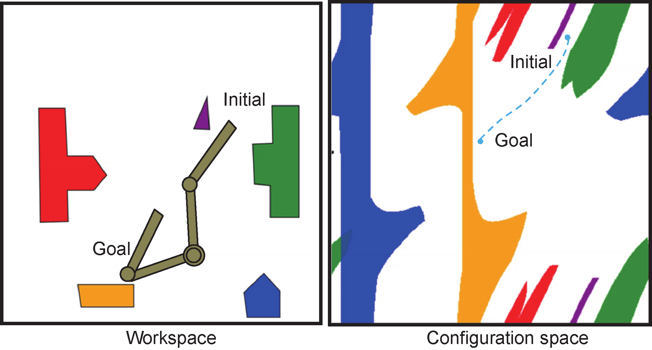
Source: Pan and Manocha, 2015.
With low-dimensional robot arms like the one pictured above, you could actually get away with discretizing the configuration space and solving an exhaustive search problem using algorithms like breadth-first search (BFS), Dijkstra’s algorithm, or A* (pronounced A-star).
For high degree-of-freedom robots, though, this will not work. Suppose we divide our joint positions into 100 for each degree of freedom: our 2-DOF arm will have a graph of up to 10000 points (less if we have obstacles), which is easy to search over, whereas a 6-DOF arm will have up to 100^6 = 1000000000000 nodes. Yikes. This is where sampling-based techniques can help to reduce the search space while still trying to cover the whole solution space. The two major classes of algorithms that exist here are:
- Probabilistic Roadmaps (PRM): This is a multi-query planner, meaning that once you generate a graph of randomly-sampled points and connect them together, you can search multiple times using that same graph. It’s a lot of up-front construction time for fast and reusable motion planning, which can be useful in static environments.
- Rapidly-exploring Random Trees (RRT): This is a single-query planner, meaning that the tree (which is a type of graph) is “grown” from the start to the goal and then discarded. RRTs, as their name suggests, are faster than building an entire PRM, but they are single-use. Sometimes, RRTs are bidirectional, meaning two parallel trees are grown from both start and goal and they are connected somewhere in the middle.
If you want to learn more about PRMs and RRTs, a good starting resource is this Motion Planning in Higher Dimensions chapter by Kris Hauser. You can also refer to the original papers for PRM and RRT for a bit of not-so-distant history.
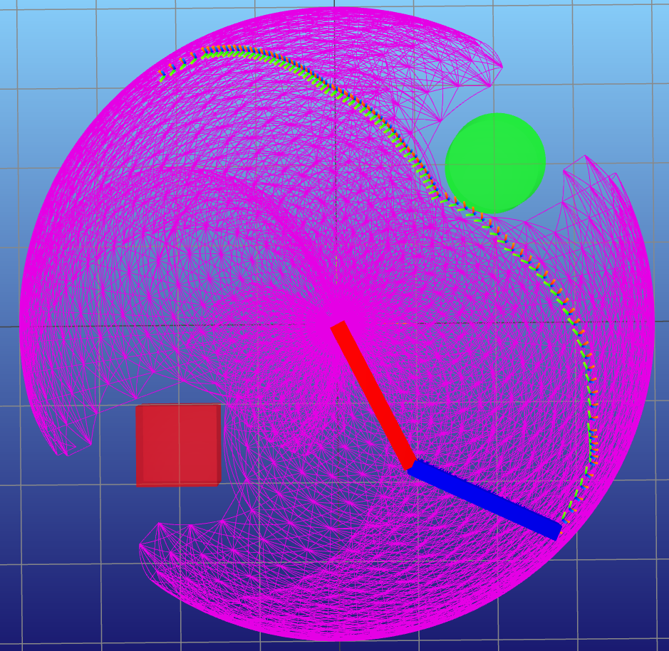
PRM (top left) and RRT (top right) results for a 2-DOF manipulator.
PRM (bottom left) and RRT (bottom right) results for a 7-DOF manipulator.
Can you even see the robot in that bottom left image?
As you can see, the paths can look… quirky. It’s a common pastime among roboticists to poke fun at the “RRT dance” that can come out from sampling-based planners. There are ways to mitigate this, but like with any sampling-based approach, there are no guarantees until you have infinite samples… so, never. Some common strategies are:
- Algorithm variants: These include RRT* and PRM* (pronounced RRT-star and PRM-star, respectively), which attempt to rewire graphs on the fly, thereby sacrificing some speed for increased path quality. These were both introduced in the 2011 paper by Sertac Karaman and Emilio Frazzoli. If you go to the Wikipedia page on RRT and head to the “Variants and improvements” section, you will find an overwhelming list of additional tweaks. Feel free to peruse this at your own risk.
- Path shortcutting: Tries to take an existing “quirky” path and sample points along it to… you guessed it… find shortcuts between those points. Some good resources to learn more about shortcutting include this section in Kris Hauser’s book, and this blog post by Valentin Hartmann.
- Optimization: I’ll save the details for the optimization section, but you can refine paths that come from a sampling-based planner using nonlinear optimization techniques.
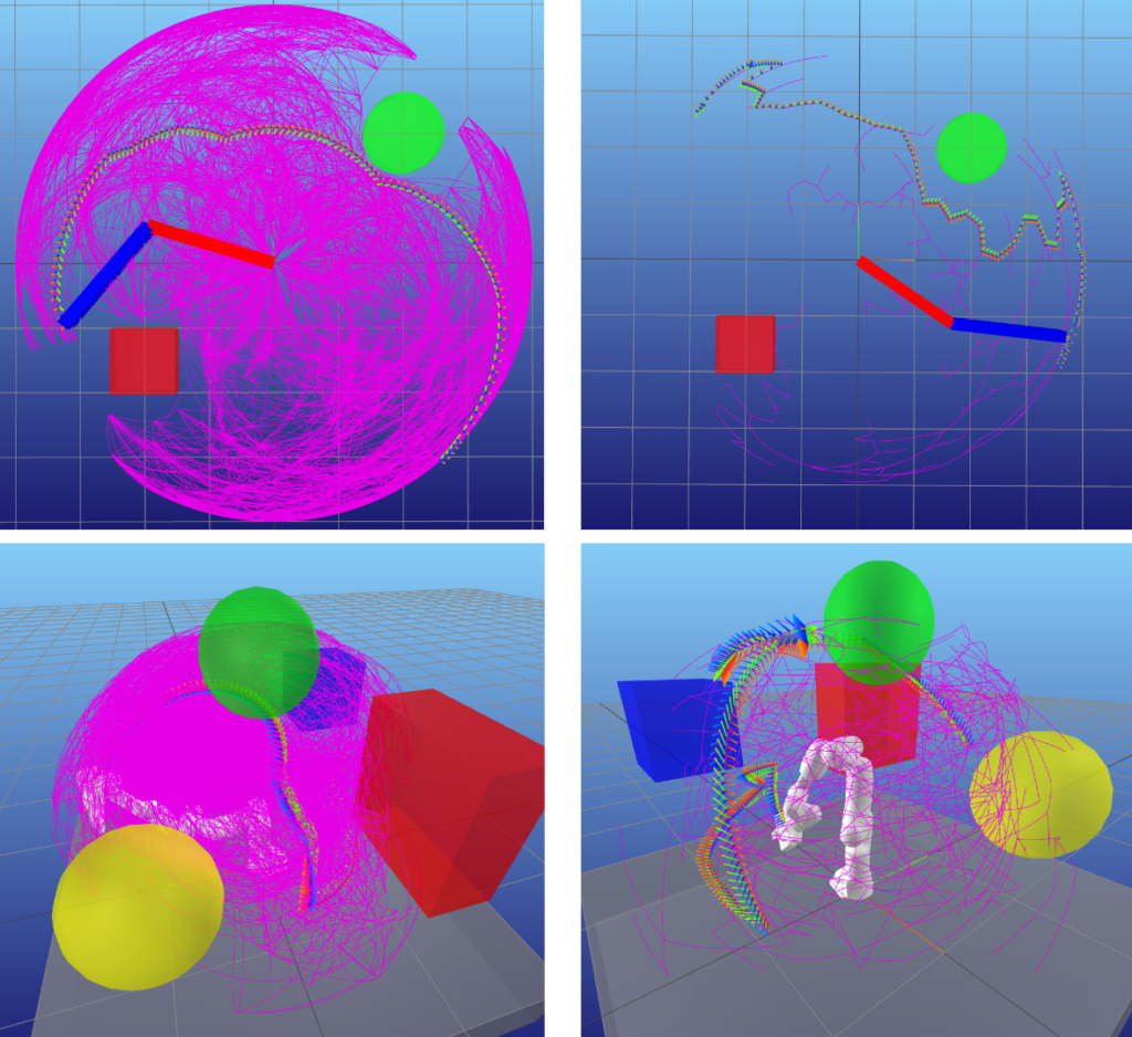
(Middle): Bidirectional RRT*. Notice how the tree is rewired to have longer branches that “fan out” from less locations, which improves path quality.
(Right): Path from a bidirectional RRT, before and after shortcutting. I’ll let you figure out which is which.
We should also talk about collisions. Motion planning requires the entire path from start to goal to be collision-free. Another complexity that arises from systems like manipulators is that collision checking also becomes more challenging. With mobile robots, for example, we can often get away with representing the robot as a circle or simple polygon (or their 3D equivalents). If both the robots and obstacle geometries are convex, you can guarantee that a straight-line segment between two collision-free configurations is also collision-free. With manipulators, one way of validating path segments is by discretizing these straight-line paths in configuration space and performing collision checks at each sample. Not only is this computationally expensive (especially if your collision geometries are full meshes), but if your sampling resolution is too coarse, or you catch an obstacle right at a corner, your planner may mislabel a path as collision-free! In other cases, you can calculate the swept volume of such geometries moving in a straight line and perform a single collision check.
Finally, it is worth highlighting that the basic implementations of these planners are purely kinematic. That is, they will produce collision-free paths, but we still need to figure out how to convert these to a trajectory that a robot can feasibly execute, sharp corners and winding paths included. There is a whole camp of kinodynamic planners that instead sample feasible motions within the kinematic/dynamic limits of what the robot can do, but in practice these tend to work only with simple systems such as autonomous mobile robots, car-like robots, or UAVs. Indeed, planners like Hybrid A* or kinodynamic RRT are used widely in these settings, but you don’t see them so much in manipulation where the combination of larger action spaces and high degrees of freedom makes them challenging to apply.
Trajectory Generation
A path tells you where to go, but not when to go. Classically, trajectory generation is the process of “timing” a path dictated by a sequence of waypoints. Whether this is a straight-line joint path or a multi-waypoint path from a collision-avoiding RRT, the same principles apply. There are various approaches to trajectory generation, each with a unique set of advantages and disadvantages.
Thanks to the laws of physics, we sadly can’t have a real robot move in a straight line at constant velocity, starting, stopping, and changing directions on a whim. We can certainly command the actuators to try and follow these glorified step responses, but this is a proven recipe for reducing the lifespan of actuators and probably getting not-so-great path tracking performance.
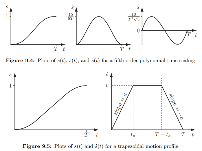
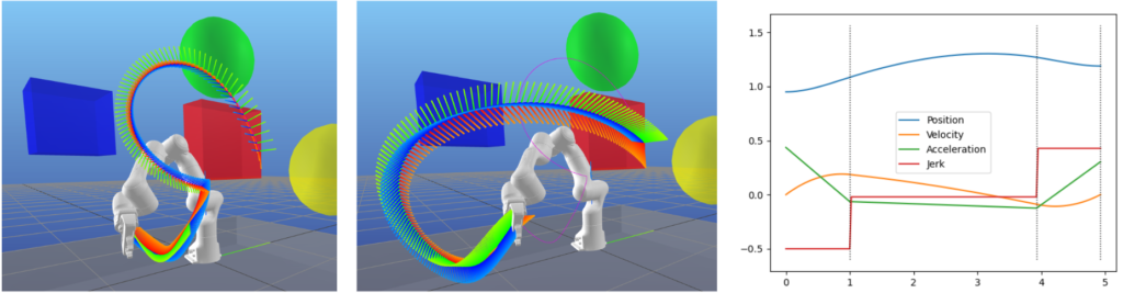
Industrial arms often rely on trapezoidal velocity profiles, also known as linear segments with parabolic blends (LSPB). These trajectories are easy to parameterize and guarantee adherence to kinematic limits because there is never any overshooting of waypoints; all segments start and end at zero velocity. However, if you look at the profile on the left image below, you will find that acceleration “jumps” discontinuously between path segments. We can fix this by augmenting the trajectory representation to trapezoidal acceleration profiles, more commonly known as s-curves (shown on the right image). The Ruckig library is the best known implementation of s-curve trajectory generation.
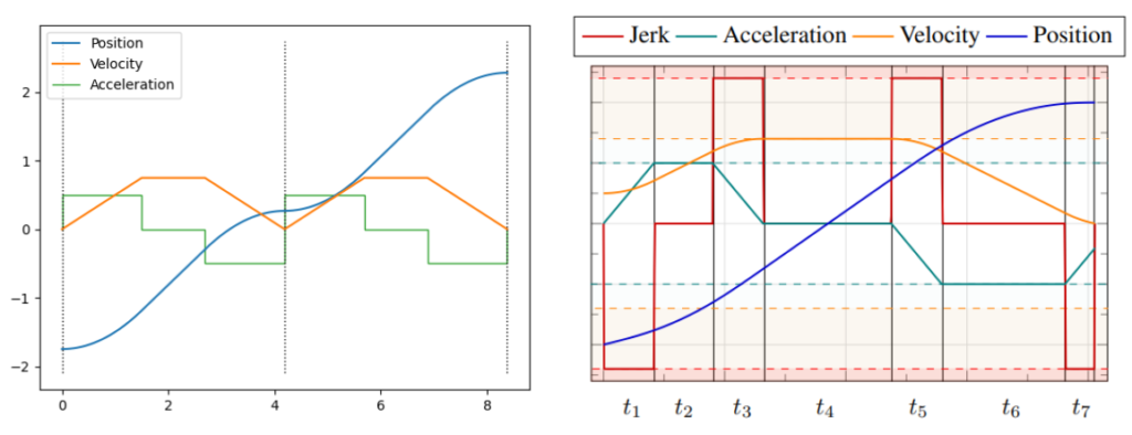
(Right) Trajectory from the Ruckig library, showing piecewise constant jerk segments. Source: Berscheid and Kröger, 2021.
The other common trajectory generation approaches involve polynomials. Polynomials have a significant advantage in that they are easy to fit, differentiable, and continuous up to their order (or degree). As shown in the next image, the most common implementations of polynomial trajectories are either cubic (3rd order) or quintic (5th order). You will sometimes hear about “minimum jerk” and “minimum snap” trajectories, which are specific incarnations of polynomial trajectories that minimize those derivatives of position. This video from an online course offered by UPenn explains the basics well.
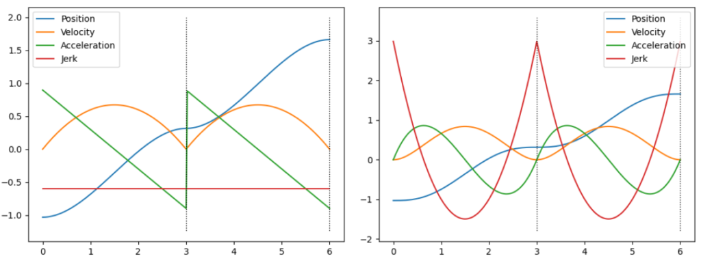
(Right) Quintic polynomial trajectory, showing more continuity at higher order derivatives such as acceleration and jerk.
Since polynomial trajectories don’t have the same constraints as trapezoidal velocity trajectories, even if boundary conditions are all safely within joint limits, there are no guarantees on the intermediate points. Other polynomial-based representations exist to address this, such as B-Splines or Bézier curves. Splines in general also guarantee smooth derivatives, but they are also defined by control points, which guarantee that all intermediate points are within the convex hull of the points (see the image below). While this comes at the expense of the trajectories being more conservative as they cannot “overshoot” the convex hull, this can be a good tradeoff to make for safety guarantees.
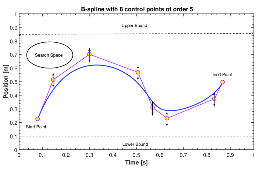
Source: Salamat et al., 2017.
Other popular approaches rely on numerical integration to compute trajectories that meet velocity and acceleration limits. Most common is Time-Optimal Trajectory Generation (TOTG), which attempts to alternate between maximum acceleration and deceleration segments while staying within kinematic limits. Here is a great explainer video for TOTG.
A related approach is Time-Optimal Path Parameterization based on Reachability Analysis (TOPP-RA). This alternates between a backward pass through trajectory segments computing reachable sets from final velocities, followed by a forward pass that picks inputs from controllable sets such that each segment ends in the reachable set of the next one. Rather than numerical integration, which can be computationally expensive, TOPP-RA generates similar trajectories by solving a set of linear programs.
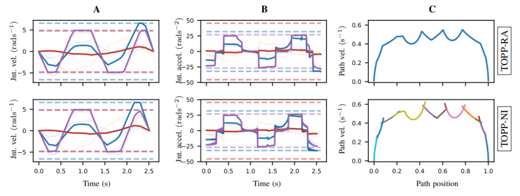
Source: Pham and Pham, 2017.
To learn more about the contents of this section, check out Chapter 9 of the Modern Robotics book. However, there are also optimization-based methods for trajectory generation that we will talk about shortly. Let’s first take a slight detour, though.
Cartesian-Space Planning
We’ve spent some time lamenting that manipulator kinematics and dynamics are nonlinear. This means that a straight line in configuration space is NOT a straight line in the real world (or in task space). So, for example, if you need your robot to follow a prescribed tool path in the real world, a slightly different approach is required.
Mathematically, the trajectory generation approaches we covered in the previous section can also be represented as a time scaling on a straight-line path.
While all the trajectories we’ve seen so far were in the joint space, nothing stops us from doing the same in Cartesian space. In Cartesian trajectories, there are 6 degrees of freedom (3 translation + 3 rotation). However, the definition of a “straight-line path” is a bit complicated due to rotation. There are two alternatives for defining such a segment.
- Constant screw motion: This couples the rotation and translation so that there is a constant twist from start to finish. You can think of this as moving along an “arc” about a fixed point in space. This approach is good in tasks like opening or closing doors, in which the screw motion can be defined about an actual hinge in the real world.
- Decoupled rotation and translation: This involves separate linear interpolation for the translational and rotational degrees of freedom. As shown in the image below, this makes the translation component be an actual straight line in task space. As such, this approach is good for tasks that require faithfully following paths in task space, including drawing, painting, or welding.
Cartesian interpolation is often done by using Lie algebra to represent the transforms (you can learn more in this tutorial). Another common approach for the rotation component is Spherical Linear intERPolation (Slerp), which is a method for interpolating quaternions developed by our good friends in the computer graphics community.
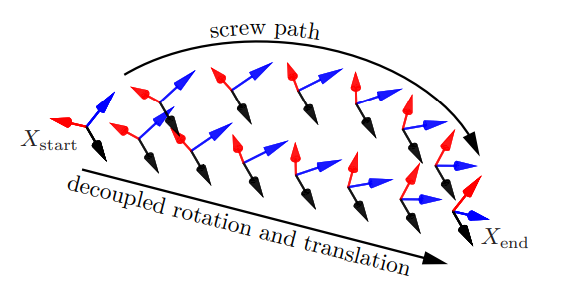
Source: Lynch and Park, 2017.
Putting it all together, you can take straight-line Cartesian paths and apply your favorite time scaling (trapezoidal velocity, polynomial, etc.) to them. As with joint space trajectories, you can similarly come up with timings that keep the resulting trajectory within specified Cartesian space velocity, acceleration, and jerk limits. My favorite resource for Cartesian trajectories is these slides from Alessandro de Luca, as they also talk about blending around corners to avoid having to stop at intermediate waypoints.
One last thing remains: To convert every step of the Cartesian trajectory to actual joint angles for our controllers. This means inverse kinematics! Luckily, the IK problem can be solved incrementally in these situations because the solution at one trajectory point is a pretty good initial guess for the next point.
There are a few more things to consider, though:
- While a Cartesian trajectory can be generated to stay within Cartesian kinematic limits, this doesn’t say much about how well the joint limits will be met after the IK step. So, you may need to do another round of validation (or even retiming). In practice, we often choose conservative Cartesian limits to maximize the chance that joint limits will also be satisfied.
- When solving IK along the entire trajectory, you can still get stuck in local minima and fail to produce a full solution. Redundant manipulators certainly help mitigate this, but sometimes you may need to rely on other techniques, such as trying with different IK solutions, or relaxing the exact adherence to the Cartesian trajectory along certain degrees of freedom (for example, maybe translation is more important than orientation).
In environments where the Cartesian constraints also need to compete with other constraints like collision avoidance, these predefined straight-line paths above may not be sufficient. Think, for example, about carrying a cup full of water over a wall without colliding. Some approaches exist that try to add Cartesian constraints to free-space motion planners. For example, this 2009 paper from Berenson et al. augments RRTs with the ability to project sampled points down to constraint manifolds, such as bounding volumes on Cartesian translation and orientation limits.
Source: Berenson et al. 2009.
Trajectory Optimization
Another way to deal with many of the motion planning problems we’ve discussed is with optimization. Generally, an optimization problem consists of a cost function to minimize, along with a set of constraints. For most robotics applications, these need to be nonlinear optimization problems since often the robot’s kinematics and/or dynamics, and complex constraints such as collision avoidance, are nonlinear functions.
The task of casting a trajectory into an optimization problem is known as transcription (as in, you are transcribing the trajectory into a nonlinear program). The two main methods you will encounter are:
- Direct transcription: This involves discretizing the trajectory into time samples. These samples are constrained with respect to each other by having to obey the kinematics and/or dynamics of the robot. While you can directly optimize over joint (or Cartesian) positions in this way, a common subclass of this approach is to instead optimize only over control inputs (forces/torques/etc.) and let the robot dynamics dictate how the positions change over time. These are known as shooting methods, in reference to shooting a cannon and letting the dynamics unfold over time.
- Direct collocation: As you may be thinking, finely discretizing a long trajectory means you may need to optimize a large number of joint (or Cartesian) points. Indeed, this can be inefficient, even if we apply shooting methods to reduce the number of variables. Collocation methods instead impose a mathematical structure on the trajectory; for example, polynomial segments. This lets us solve optimization problems over a much smaller number of decision variables, such as the boundary conditions of the segments, or the polynomial coefficients themselves.
In practice, direct transcription methods are more often applied for short-horizon control, whereas collocation methods are used when converting full paths to trajectories.
One of the best resources on trajectory optimization is this set of tutorials from Matthew Kelly, who currently works on the Atlas humanoid robot at Boston Dynamics. Russ Tedrake’s Underactuated Robotics course also has a great chapter on trajectory optimization.
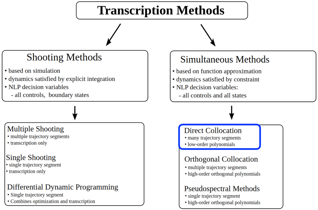
(NLP = non-linear program).
Source: Matthew Kelly, 2016.
Some common transcription based implementations that have made their marks in robotics include:
- Covariant Hamiltonian Optimization for Motion Planning (CHOMP), by Ratliff et al. (2009). Uses gradient descent to optimize points in a trajectory while satisfying constraints such as collision avoidance.
- Stochastic Trajectory Optimization for Motion Planning (STOMP) (Kalakrishnan et al., 2011) and Incremental Trajectory Optimization for Motion Planning (ITOMP) (Park et al, 2012). These are gradient-free methods that rely on generating noisy trajectories — hence stochastic — to similarly optimize while satisfying constraints.
- The TrajOpt framework from Schulman et al. 2013) uses sequential quadratic programming (SQP) to perform trajectory optimization. In my opinion, this brings us into what I would consider “modern” approaches at the time of writing. TrajOpt has been adopted by several software packages, most notably by Tesseract as part of the ROS-Industrial initiative. See this post for more information.
Source: ROS-Industrial, 2018.
For direct collocation approaches, perhaps the best known offering is found in Drake. Drake offers DirectCollocation and KinematicTrajectoryOptimization classes, which perform direct collocation with cubic spline and B-spline parameterizations, respectively. In Drake, you can add arbitrary constraints to mathematical programs, which means you can augment the above problems with your own constraints for kinematic/dynamic limits, position/orientation limits, collision avoidance, and more.
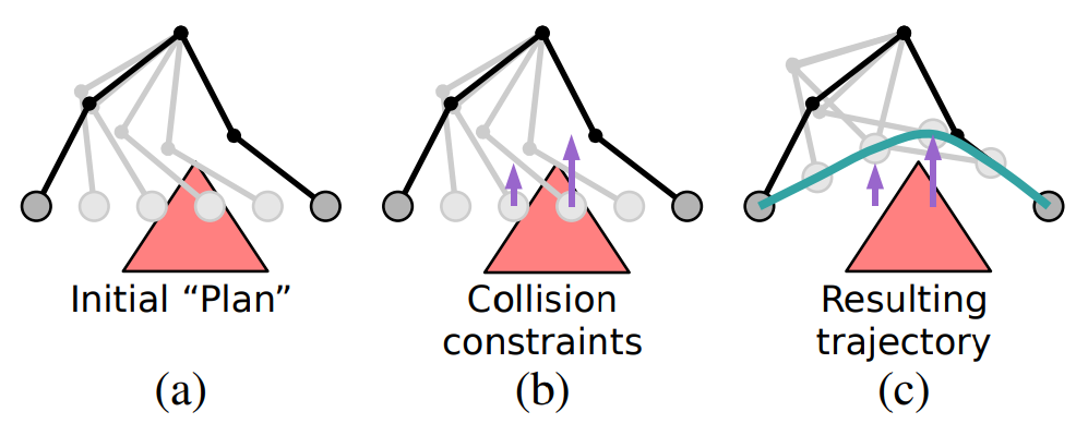
Regardless of which optimization method you choose, a simple technique that can work well is to use the simplest possible “path planner” as an initial guess. That is, assume a straight-line path with evenly spaced waypoints, and let the optimizer squash away all the constraints that may be violated.
Source: Kolter and Ng, 2009.
Adding collision avoidance constraints to either IK or trajectory optimization was something that took me a long time to figure out. As such, I want to expand on it here in case you are similarly confused. Using the diagram below as a guide, the high-level idea is:
- Find a vector representing the collision (or near-collision). If you have simple shapes like spheres or capsules, you can find this analytically. Otherwise, you can rely on your favorite collision checking library to give you a pair of points.
- Find the parent joint(s) of the contact point(s). In our diagram, for example, the contact point on the arm (
p1) is parented to the second joint. That is, the transform between the parent joint andp1is a rigid transform that does not depend on any joint positions. - Compute the Jacobian at both the contact points. This is done by transforming the Jacobian at the parent joint with the additional rigid transform between the joint and contact point. This is referred to as the contact Jacobian.
- Define the gradient. In our example, the gradient will use the contact Jacobian to move the first two joints in the direction opposite to the collision distance vector. If
p1andp2both happen to be on moving parts of the robot (so it’s a self-collision check), you can push both points away from each other using two separate contact Jacobians!
With this information, if you want the real mathematical details, check out section IV of the TrajOpt paper (Schulman et al., 2013) and section III of this paper by Chiu et al., 2016.
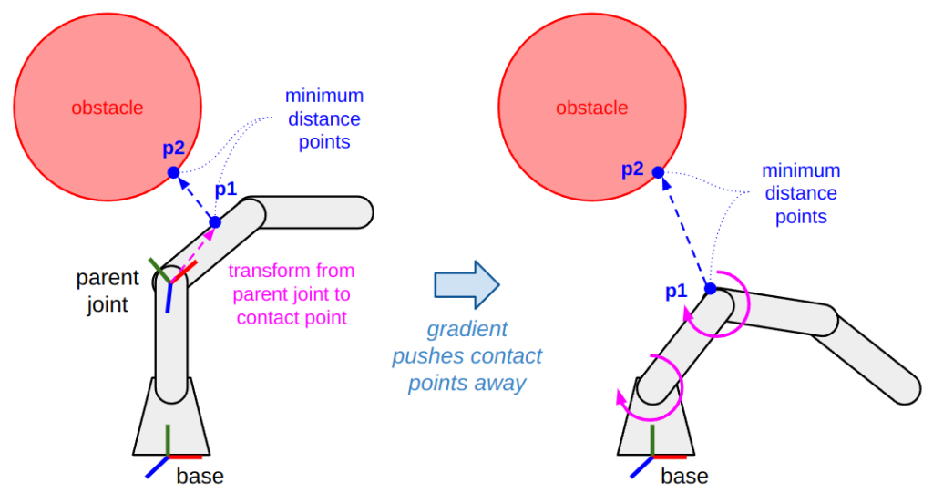
The key is to find contact points and a vector between them, which can dictate how to move the joints to increase the distance between these points until the constraint is satisfied.
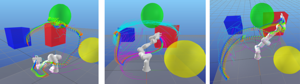
Unfortunately, nonlinear optimization is also quite sensitive to initial conditions. While a straight-line path as an initial seed can be effective, it breaks down with complex environments full of obstacles. One common remedy is to use a real path planner after all. For example, you can generate a suboptimal path using an RRT, and then improve it with optimization.
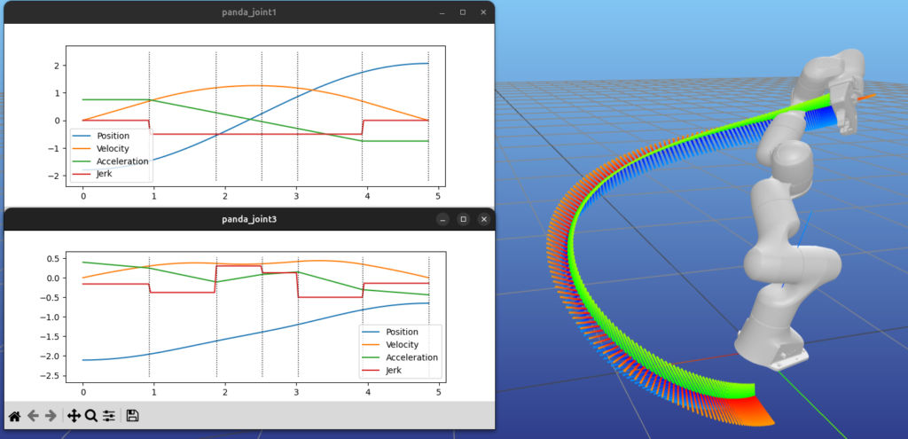
(Middle) Resulting trajectory after optimization.
(Right) The cubic polynomial segments of the optimized trajectory for one of the robot’s joints.
Other state-of-the-art approaches try to combine the best of both worlds: search and optimization. One of the most promising is Graph of Convex Sets (GCS) from Russ Tedrake’s group, first introduced in 2021. GCS first does a (computationally expensive) pre-processing step that decomposes the environment into convex components. Then, it applies graph search to find paths through this graph of convex sets from the start to the goal component. Within each component, you can perform an optimization to get physically consistent trajectories. Because the graph components are convex, and they have chosen B-Splines for their direct collocation method, they can guarantee that each trajectory segment will stay inside the convex set! Cool, right?
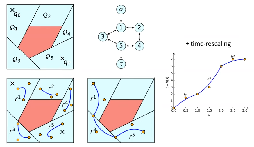
Source: Russ Tedrake, 2023.
Motion Planning in the Bigger Picture
… and there you have it. All of motion planning is solved and neatly wrapped up for you.
Of course, I’m joking. There is so much more that we didn’t cover, which is why robotics is as exciting as it is overwhelming.
In this next section, I want to talk some more about what happens “above” and “below” the motion planning components we’ve introduced. Specifically, what is the relationship between motion planning, perception, and control? How are different kinds of sensing applied to give our motion planning stack its mythical “point B” to plan towards, and actually execute it in real-world tasks that may involve contact or other unanticipated information about the environment?
There is also one more piece that fits “above” motion planning, which is to combine it with higher-level task planning. This is referred to as task and motion planning (TAMP), and I have another blog post on this topic if you want to learn more.
Motion Planning and Control are Intertwined
So far we’ve spoken about motion planning as a deliberative, “point and shoot” type approach: you plan a path, convert it to a trajectory, and wait for that whole trajectory to finish executing. This is not necessarily feasible in highly dynamic or uncertain environments, in which reactive replanning may be necessary. This type of anytime motion planning is defined as first producing a feasible solution, and continuously refining it during execution. Indeed, in the same year that they introduced RRT*, Karaman et al. (2011) were already thinking about anytime motion planning.
I said I wouldn’t talk much about low-level control in this post, but there are some important points to make here. While you can use path planners in an anytime fashion, you can also close the feedback loop closer to the control layer. Critically, lower-level control loops are faster than path planning loops, so they are more naturally suited for reacting to dynamic obstacles, external disturbances, and so on.
One common application of anytime motion planning is teleoperating or servoing a robot manipulator. Servoing often involves commanding a coordinate frame on the manipulator, like the end effector, to move in a specified task space direction. One example is using a gamepad (or similar device) to give operators six-axis control of the arm’s motion for manual correction or failure recovery. Lately, these approaches have also become crucial in collecting data for, and autonomously executing, learned policies that executes Cartesian velocity commands directly from visual feedback.
Indeed, manipulator servoing can be framed as an anytime version of inverse kinematics, where we can use the Jacobian to convert a task space velocity or target pose command to joint velocities that the robot can track in a loop. As we saw in the IK section, this “single step of IK” can similarly be augmented with nullspace projection tasks for joint limit adherence, collision avoidance, etc.
Perhaps it’s not surprising that trajectory optimization can also be used in an anytime fashion. Notably, direct transcription methods directly turn into Model Predictive Control (MPC) if you slap a finite time horizon and feedback loop on them. Today, most state-of-the-art control methods for high degree-of-freedom systems (like manipulators and legged robots) apply some combination of nonlinear MPC and machine learning (usually imitation and/or reinforcement learning). Leading experts in these areas include Boston Dynamics and the Robotic Systems Lab at ETH Zurich.
These are just a few examples. All I want to get across is that motion planning began with easier problems, assuming the world is perfectly observable and controllable, and that only the agents involved in planning can change the state of the world. However, as the robotics field has got better at solving these problems, it naturally turns towards more complicated environments where reactive planning and control is necessary.
Don’t robots have to, like, grab and push stuff too?
They certainly do! Let’s think of a few other tasks: inserting a cup in a holder, wiping a table, turning a door handle, or tightening a nut on a bolt. All these problems have something in common: they require making contact with the world.
Figuring out how to grasp an object first depends on the type of end effector that the robot has. Common categories of end effectors include parallel-jaw grippers, vacuum grippers, multi-finger grippers, as well as task-specific tool ends. Some robots that need to perform a variety of tasks have swappable end effectors, in contrast to the more research-oriented line of thinking claiming that a single, general-purpose dexterous hand can do the job.
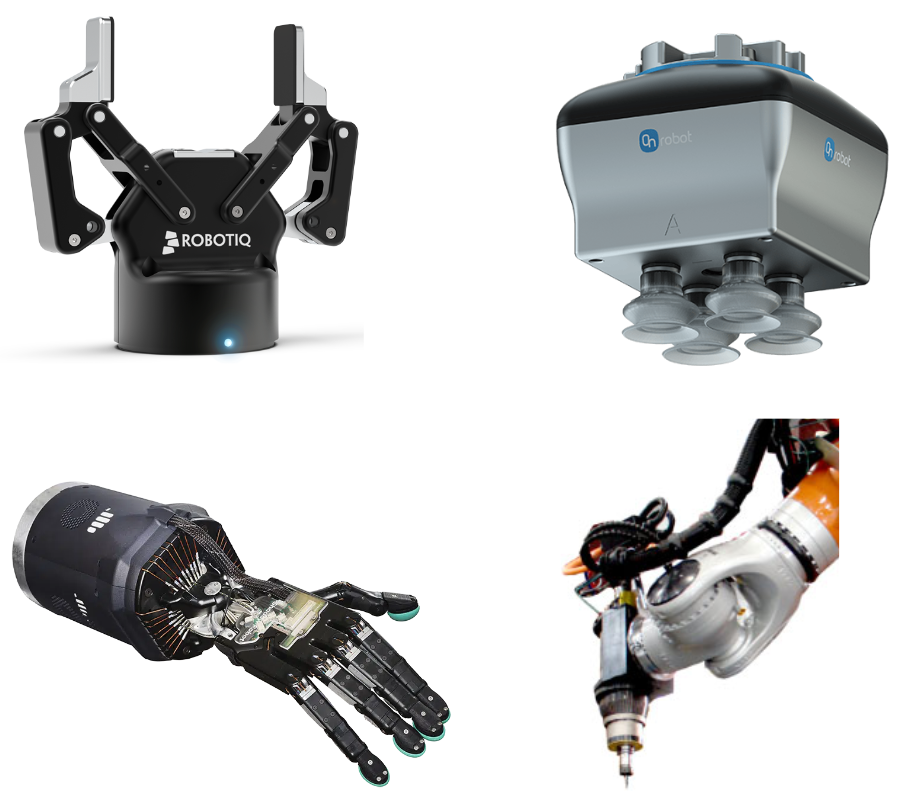
(Top left) Robotiq 2F-85 parallel-jaw gripper.
(Top right) OnRobot VGC10 vacuum gripper with 4 suction cups.
(Bottom left) Shadow Dexterous Hand with 5 fingers and 20 degrees of freedom!
(Bottom right) Drill and tapping end effector system mounted on a KUKA industrial arm, from ARC Specialties.
Next, we should talk about sensing contact. Some manipulators have joint torque sensors which let you calculate what the robot is “feeling”. For example, if a dynamics model of the robot indicates a joint should measure 10 N of force, but it is actually seeing 5 N, then there is something pushing up on the arm (or the sensors are bad). These sensors are relatively inexpensive since they are probably needed by existing low-level controllers anyway. However, they are prone to “blind spots” in certain configurations where a robot may not be able to measure any force/torque along some directions. Other systems have 6-axis force/torque sensors, which are more expensive but better behaved in that they don’t have such blind spots and don’t require an accurate dynamics model of the robot.
Why do we need force/torque sensing? These sensors, combined with good control algorithms, lets your robot behave less like a rigid system that knocks over everything in its fixed path, and more like a compliant system. Compliance is necessary for tasks that require establishing and maintaining contact with the environment, such as wiping or sanding surfaces, or “peg-in-hole” insertion. These methods, such as impedance control and admittance control, are frequently applied for such tasks. It is also generally good that a robot can be compliant for safety considerations, especially around humans, which is why most collaborative robots (or cobots) have some flavor of compliant control built in.
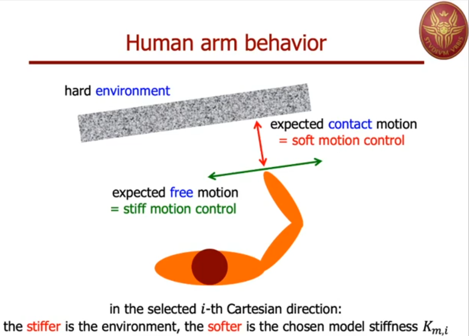
Source: Alessandro De Luca, 2020.
Of course, it’s not just the arms that require sensing. End effectors themselves can be (and are) similarly equipped with force and/or pressure sensors to detect contact. This can serve many needs, like avoiding damage when handling objects, or exerting forces for tasks that require it, like pushing buttons or flipping switches. It doesn’t stop there, though; robots can be (and are) outfitted with new sensing modalities that humans and animals don’t directly have, such as wrist cameras or time-of-flight sensors to detect proximity to objects before actual contact is made.
We also shouldn’t diminish the passive solution to these grasping problems, which gets back into soft robotics. There are countless compliant end effector designs, from the relatively common fin ray effect and soft silicone grippers to the more esoteric jamming and entanglement grippers, to name a few. Of course, you can always introduce compliance in both the mechanical design and the underlying software.
Connecting Perception and Motion Planning
Before we can perform the contact-rich tasks we just described, it’s also important to know what the target objects look like, and where they are in the world. We’ve mentioned moving from “point A to point B”, but how do we know what “point B” is in the first place? There are various perception methods for identifying objects, or affordances on objects, that enable manipulation tasks. These include:
- Making objects easy to detect: Some simple approaches include using colors that are easy to identify with cameras (like a bright orange ping-pong ball), adding reflective markers compatible with motion capture (mocap) cameras, or fiducial markers (ArUco markers, AprilTags, etc.). These approaches are used often in prototypes where perception is not the focus of the work being demonstrated, but also exist in commercial applications such as warehouse automation or robot docking stations where a little bit of environment modification goes a long way for reliability.
- Geometric methods: Using point cloud data to fit basic primitives (cuboids, ellipsoids, etc.) around objects, then figuring out how to grasp them. This often requires making strong assumptions about the environment, such as a flat tabletop plane with well-separated objects that can be processed exclusively with geometry-based methods.
- Registering against a known model: Using point cloud registration techniques like the Iterative Closest Point (ICP) algorithm, you can use a ground truth model of an object (for example, from a CAD drawing) to locate objects. These methods can be quite robust, but getting models for every object you want your robot to manipulate is sometimes challenging, or even impossible, depending on the application.
- Machine learning: This is a massive solution space, but in the context of finding objects for manipulation there are two main categories. Firstly, you can use object detection models to segment out individual objects in a scene. These could be task-specific models trained to detect specific object types, as I describe in this blog post, or foundation models trained on massive datasets, such as Segment Anything. On the other hand, there are model categories like DexNet that can directly output grasp candidates without the need to identify individual objects. Professor Rob Platt (who, incidentally, is my current manager) has a great 2022 survey paper on these methods.
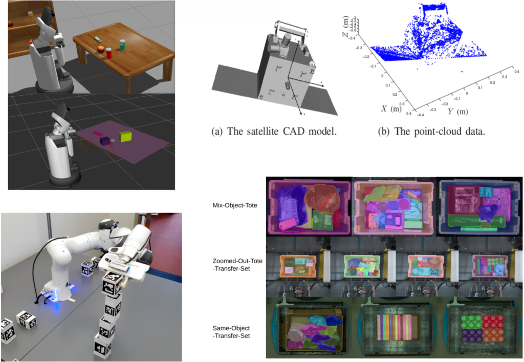
(Top left) A tabletop perception scene which segments objects from a tabletop and fits cuboids around them.
(Top right) An example of point cloud registration for grasp detection (Source: Aghili, 2012)
(Bottom left) A block stacking application which uses fiducial markers for accurate detection (Noseworthy et al, 2021).
(Lower right) Learned object segmentation for bin picking applications (Amazon Robotics, 2023)
Software Tools for Motion Planning
If you want to get hands-on with this material and actually implement motion planning systems, what software packages should you turn to? Many of these have already been mentioned throughout the post, but I felt it useful to dedicate a whole section to better organize the motion planning software space.
For modeling robot kinematics and dynamics, my top choices are Pinocchio, Drake, and MuJoCo. They are all modern and actively developed frameworks, developed in C++ but exposing first-class Python bindings. Other tools you may see out there are Peter Corke’s Robotics Toolbox for Python and MATLAB’s Robotics System Toolbox. Expectedly, all these tools can ingest URDF files which allows for interoperability with the actual design.
For collision checking, libraries include Bullet and Flexible Collision Library (FCL) (used in MoveIt, Drake, and Tesseract). The Pinocchio authors created their own variant and improvement of FCL named HPP-FCL. Fun fact: the HPP stands for Humanoid Path Planner, and not the extension for C++ header files… but that’s fine because it’s being renamed.
Going back to my “top 3” libraries for model representation: One way to choose which tools you should consider is how they connect to motion planning.
- Pinocchio does not have any direct support for motion planning, as it is designed to enable the development of planning and control algorithms. There are some amazing open-source optimal control packages built on Pinocchio, like Crocoddyl and OCS2.
- MuJoCo is more of a modeling and simulation framework, so it also doesn’t offer much planning functionality. There are some nice examples by Kevin Zakka that show MuJoCo for robot manipulator control and inverse kinematics. At the time of writing, MuJoCo is about to release support for signed distance fields (SDFs), which is something else to consider.
- Drake has several built-in motion planning algorithms, but they generally bias towards the work of Professor Russ Tedrake’s research group at MIT and Toyota Research Institute. Drake offers state-of-the-art optimization-based inverse kinematics and trajectory optimization implementations, as well as Graph of Convex Sets (GCS). It also has some high-fidelity hydroelastic contact modeling support for simulation use cases.
Other popular software libraries are less about modeling and more dedicated to motion planning. These include:
- Open Motion Planning Library (OMPL): A C++ based library (with Python bindings) for sampling-based motion planning. It was implemented by Willow Garage and Rice University and published in 2012 to support high degree-of-freedom robots such as Willow Garage’s famous PR2 robot. OMPL implements an astonishing amount of sampling-based planning algorithms, which makes it appealing for benchmarking and design exploration. Despite its age, OMPL is still maintained and remains the standard for sampling-based planning.
- MoveIt: The de facto motion planning framework for the ROS ecosystem, originally developed at Willow Garage, also for the PR2 use case. It is mainly known for sampling-based motion planning since it wraps OMPL due to Ioan Șucan’s involvement in both projects. However, MoveIt offers a plugin-based system for integrating other inverse kinematics, motion planning, motion adapter, and collision checking algorithms. While MoveIt can sometimes suffer from the same aging woes as OMPL, it is still being maintained and remains the most tightly connected to ROS. If you are using a robot that runs ROS, you may want to give MoveIt a look.
- Tesseract: Another ROS based motion planning framework developed by Southwest Research Institute, key players in the ROS-Industrial consortium. It shares a lot of its design philosophy and concepts with MoveIt, but it is a newer software package. This means that, while less popular at the time of writing, the authors have had the chance to correct for some of the drawbacks they identified in MoveIt, such as better decoupling of core functionality and ROS, and through this more “proper” and easy-to-use Python bindings. Tesseract also has the best current support for TrajOpt.
- cuRobo: A relative newcomer from NVIDIA, in the form of a full motion planning stack that takes as much advantage of GPU acceleration as possible to show really compelling results (and sell RTX cards). It uses the nvblox library for GPU-accelerated signed distance field computation, but also implements highly parallelized inverse kinematics, trajectory optimization, and collision checking. It is included in the NVIDIA Isaac Manipulator package, meaning it is well integrated with Isaac Sim and Omniverse.
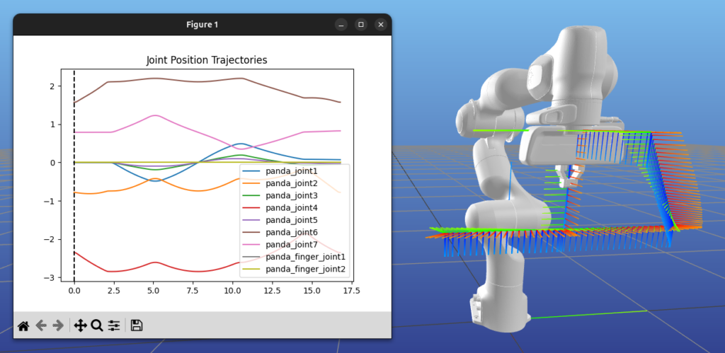
A lot of these tools are extremely capable, but in my opinion they are not very welcoming to newcomers. This is why I created PyRoboPlan, which is where several screenshots in this post come from. It is built using the Pinocchio Python bindings, but all the motion planning algorithms are developed from scratch with a goal of being easy to understand and modify, and not so much on performance. I would appreciate that you check it out, run the examples, and help teach yourself motion planning this way! I would also very much appreciate feedback and contributions.
Conclusion
As you have seen, motion planning for robot manipulators is a complex field that is still evolving every day. I find it very exciting, and maybe a little disappointing, that a decade from now this post will require significant revisions or may be entirely obsolete. How true this projection holds up depends on you, the readers, to move this field forward. I hope I’ve done my part by removing some of what may be intimidating you into giving it a try.
If you want to get more into the mathematical foundations of motion planning, I’d like to share some of my go-to resources:
- Modern Robotics by Kevin Lynch and Frank Park: This is an amazing educational resource which includes a free book with exercises and top-notch accompanying videos that were part of a Coursera course. Easily my favorite for learning the foundations.
- Robotics Systems book by Kris Hauser: Contains two of my favorite references on Inverse Kinematics and Motion Planning in Higher Dimensions (sampling-based planning). Definitely take a look beyond just the chapters I’ve pointed out.
- Robotic Manipulation course by Russ Tedrake: A free online book with annually recorded video lectures and awesome interactive notebooks you can run directly on the web. Compared to the other materials I’ve selected, this course maybe glosses over some of the basics and leans more towards Professor Tedrake’s own software (Drake) and research expertise in optimal planning and control. You may also benefit from his other course, Underactuated robotics; especially relevant to this post is the trajectory optimization chapter.
- Trajectory Optimization tutorials by Matthew Kelly: Great if you want even more detail on trajectory optimization methods.
- QUT Robot Academy videos by Peter Corke: There are more great resources here on several topics, but I especially like the way Professor Corke explains spatial mathematics and robot kinematics. While this post only described kinematics as transformation matrices, there are other concepts like Denavit-Hartenberg parameters and Lie algebra you might want to learn about with these resources.
If you have any questions, corrections, or any other reason to reach out, I would be happy to hear from you. Also, I have to be shameless and again promote my tool PyRoboPlan. Please try it out and contribute if you can!
Thanks to the great people who helped review and improve this post:
José Avendaño, Sebastian Jahr, Bill Mather, Andy Park, and Sam Pfeiffer.
Thanks Sebastian for this great post!
I am an embedded software engineer by trade but I have a background in control theory and I am now moving my career towards robotics (I actually started following the Modern Robotics lectures a couple of months ago).
Reading this article has clarified how all the parts are fitting together and given me additional resources to look at!
Thanks for writing this and putting all these resources in one place!
Been doing robotics for over 20 years. This is a brilliant effort at a review of what’s out there. Well done.
I come from a robotics perception background, and this has been a great read to better understand how all the lower sub-systems work, how they fit together, and how to find further resources for them. Thanks a lot for taking the time to write such a long and well articulated post!
Vergy good post!! I really wished to learn motion planning, but I couldn’t find some suitable materials or tutorials with example codes. I will follow your “pyroboplan” package in order to catch a concept of the motion planning (Actually, I didn’t understand well robot arm motion planning in 3D space (especially, when checking collision: relationsphis between robot arm shape, configuration space, RRT/PRM, how/and what to check collision ..)) 2D case is quite intuitive and understandable. But, I don’t know why most of books or materials only shows 2D images even when explaining motion planning for (6 dof) robot manipulator. (Not easy to me)
Anyway thanks for your good post !!!
Again great job Sebastian! I always learn something new and identify a gap in my robotics knowledge whenever I read your posts. I can not imagine the amount of effort got into this post. Thanks a lot!
Great blog! I’m really looking forward to the next post, and thank you so much for your dedication!
Thank you very much to the author for sharing. I am an ordinary university student, and I have been interested in learning more about robotics. Previously, I did a lot of unrelated work, but after reading the author’s blog, I have benefited greatly. It has clarified the methods and approach to learning. I hope that in the future, I can achieve success in this field.
this is amazin. thank you
Greatly appreciated for your efforts. Excellent work!