
In this post we will go through the process of training neural networks to perform object detection on images. I’ll be discussing some software I used for my current work, which include the COCO Annotator tool for annotating data and the Detectron2 library for training and using models.
I’ve taken a chunk of data, filtered down some of my code into Jupyter notebooks, and put them in this GitHub repo so you can follow along.
Introduction (and Unintentional History Lesson?)
It should come as no surprise by now that machine learning — specifically, the use of deep neural networks — has taken over computer vision in the last few years. Results have been outstanding because it’s extremely hard to write down mathematical rules by hand that operate on high-dimensional visual data such as thousands of pixels on an image to recreate natural intelligence. Therefore, having a computer learn patterns from large datasets is a suitable solution.
Machine learning works great for computer vision because we have not (yet) figured out something better that we can fundamentally understand.
The pivotal moment of the machine learning takeover was arguably the unveiling of AlexNet in 2012, which showed a significant year-over-year improvement in results on the (then active) ImageNet Large Scale Visual Recognition Challenge (ILSVRC). Many of the standard convolutional neural network (CNN) architectures we practitioners take for granted nowadays were winners of this challenge until it ended in 2017. One that will come up in this blog post is Residual Networks (or ResNets) which similarly were the headliners in the 2015 version of the ILSVRC.
If you want to dig into the theoretical background, I would highly recommend Justin Johnson’s Deep Learning for Computer Vision course at University of Michigan. It’s fantastic. If you want just enough for this blog post, watch the object detection lectures (15 and 16) in this YouTube playlist.

Source: Deep Learning for Computer Vision — Lecture 15, Object Detection, Justin Johnson (2019)
For one of my projects at MIT this year, I needed to quickly stand up some neural networks that could perform basic object detection for home robotics tasks. I decided to use the Detectron2 software library from Facebook AI Research (FAIR), which came out fairly recently in 2019. Detectron2 has a “2” in it because it is FAIR’s official backend switch from Caffe to the (today) more ubiquitous PyTorch.
FAIR has been responsible for publishing several novel neural network architectures for computer vision tasks. Two popular ones you may have heard of are RetinaNet for bounding box detection and Mask R-CNN for instance segmentation.
Now that you (maybe) read this section let me add some more detail. In the rest of this post, I will describe how I went about collecting image data for home service robotics tasks, annotating the data, and training both RetinaNet and Mask R-CNN object detectors using Detectron2.
NOTE 1: I am in no way affiliated with FAIR or Facebook in general. I simply use their open-source tool and it has worked great for me. This is me giving back by writing a brief tutorial to help others should they want to get started with Detectron2.
NOTE 2: It is no coincidence that Kaiming He is a lead author in the ResNet and the Mask R-CNN papers, and at the time of this post is affiliated with FAIR.
Collecting and Labeling data
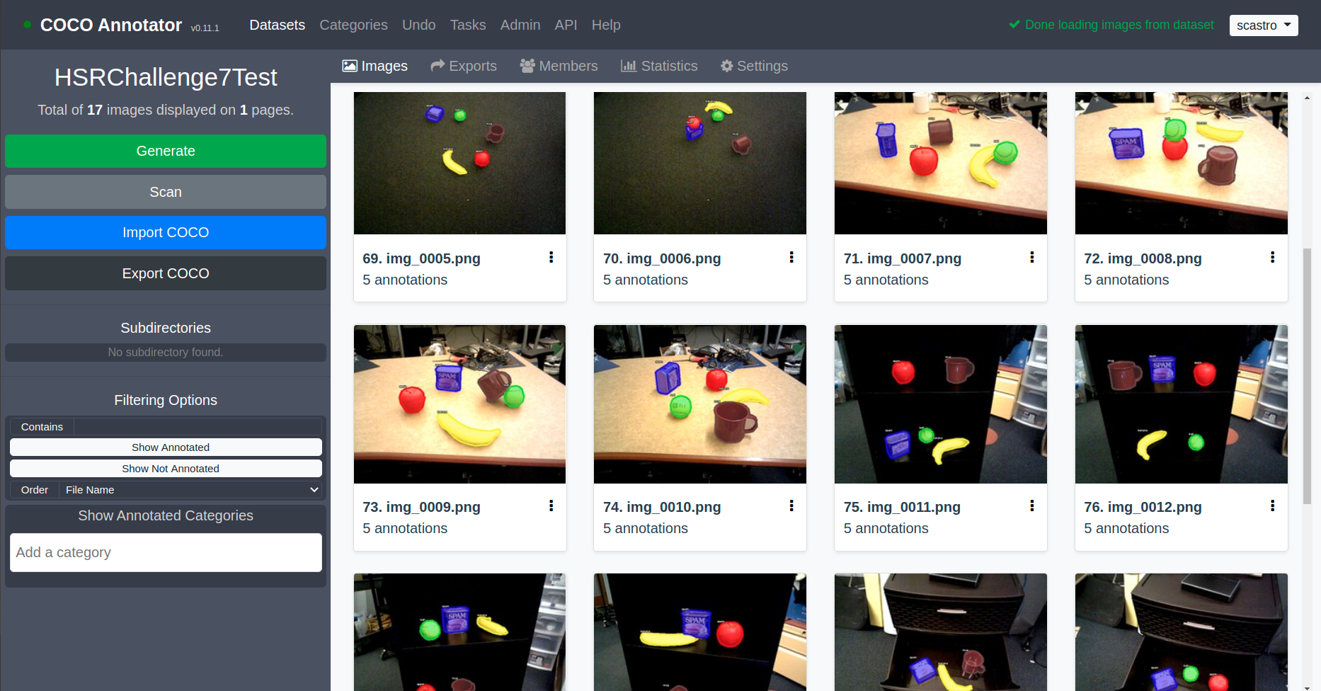
For the example I shared on GitHub, I collected real camera data from my beloved Toyota Human Support Robot (HSR). I drove the robot around a couple of viewpoints in the lab as shown below. Since this robot uses ROS, it was fairly straightforward to stream images and save select ones as image files. For simplicity, I chose 5 object categories: Apple, Banana, Mug, Spam, and Tennis Ball.

Once we have a set of images, next comes the “fun” task of labeling them. Seriously: if you have a way to automate data labeling, it’s generally worth the effort unless you have a good (and ethical) crowd-sourcing platform at your disposal. Simulation, especially in photorealistic simulators, has proven to be helpful. One recent example is NVIDIA’s Deep Object Pose Estimation (DOPE).
Luckily, this problem is simple enough that I only spent a few hours manually labeling a small batch of data. The sample dataset has 64 images (320 annotations) for the training set, and 17 images (79 annotations) for the test set. This was sufficient at least for running experiments within my constrained lab setting. Typically you want on the order of thousands of datasets, especially if you’re training a model from scratch.
Supervised learning is not picky about the format or approach you choose for data labeling, and therefore there are LOTS of tools out there. This post summarizes a few of the key ones you may have seen floating around.
The tool I selected was COCO Annotator. Justin Brooks, the developer of the tool, was super helpful and approachable, so I would be remiss to not plug his newer and more professional undertaking: DataTorch. While COCO Annotator is good enough for quick local projects, tools such as DataTorch tie into cloud storage which is useful for scaling up to a more realistic project where multiple users are involved.
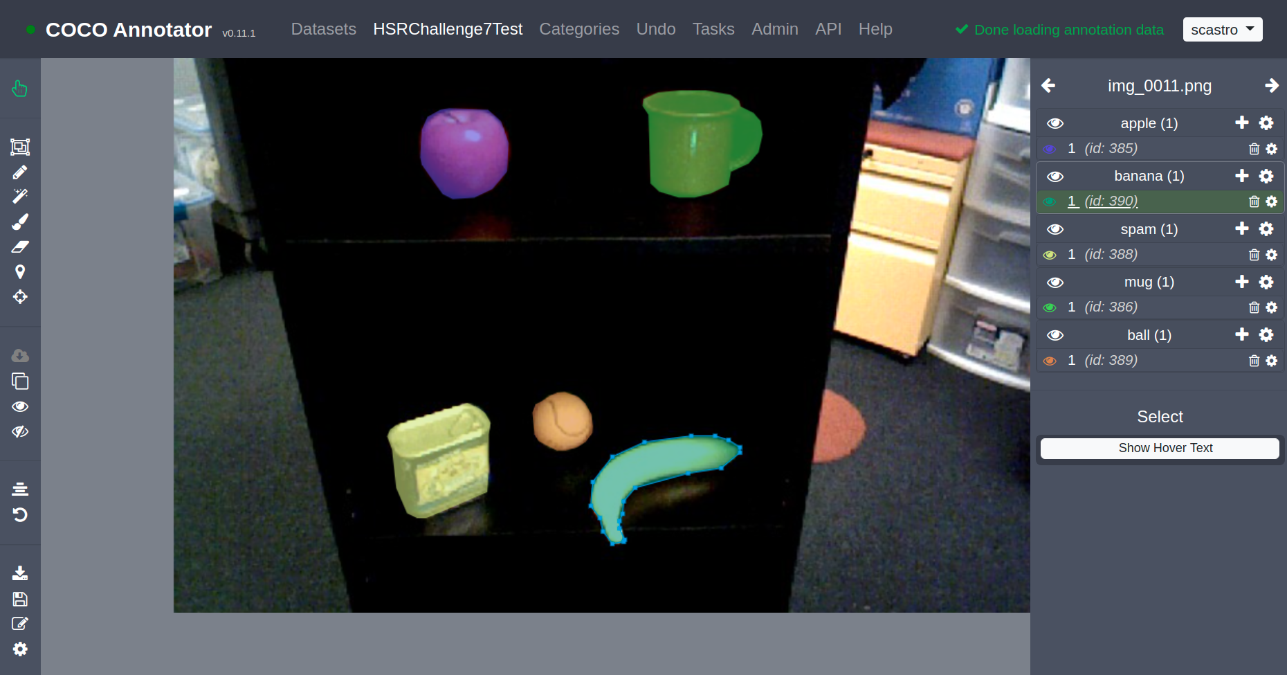
This labeling tool gets its name from the well-known Common Objects in COntext (COCO) benchmark dataset. In addition to the dataset itself, COCO uses JSON to represent all the annotation metadata associated with images (i.e. the labels). So annotation tools like COCO Annotator will export to the COCO format and machine learning frameworks like Detectron2 will similarly consume the COCO format. Furthermore, there are official COCO APIs for scripting in languages like Python, MATLAB, and Lua. Yay.

If you expand “segmentation”, you get all the pixels comprising an image mask, so I left that one collapsed 😉
Using a Pretrained Model
Detectron2 provides a set of baseline models which include standard model architectures, datasets, and training schedules. These are all contained in their Model Zoo. To bring things full-circle from the introduction:
- All their baseline models are trained on the COCO dataset.
- RetinaNet and Mask-RCNN are model architectures born out of FAIR so you will see them heavily featured in the Model Zoo, but there are other models available and one would expect to see more over time.
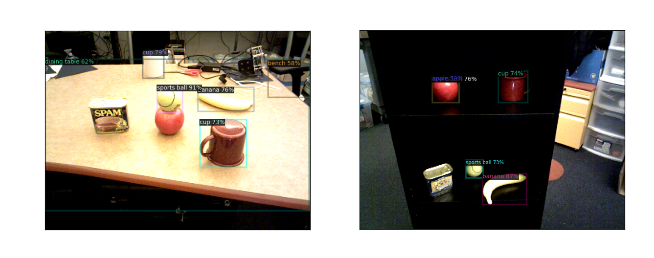
In our first example, we will directly use pretrained models from the Model Zoo and see how they perform on our dataset. The bare-bones code below will set up a pretrained Mask R-CNN network with a ResNet50 base and create a predictor that returns all detections with a score over 0.5 (or 50%).
from detectron2 import model_zoo
from detectron2.config import get_cfg

# Create a configuration
cfg = get_cfg()
model_file = "COCO-InstanceSegmentation/mask_rcnn_R_50_FPN_3x.yaml"
cfg.merge_from_file(model_zoo.get_config_file(model_file))
cfg.MODEL.WEIGHTS = model_zoo.get_checkpoint_url(model_file)
cfg.MODEL.ROI_HEADS.SCORE_THRESH_TEST = 0.5

# Create a predictor using the trained model
from detectron2.engine import DefaultPredictor
predictor = DefaultPredictor(cfg)
Next, we can use this predictor to infer on images. Here, I am loading the images with OpenCV, and Detectron2 has its own visualizer that annotates them. The GitHub examples use Matplotlib to display code so the images show up in Jupyter notebooks, but if you’re running locally a standard OpenCV window will do.
import os
import cv2
import matplotlib.pyplot as plt
from detectron2.utils.visualizer import Visualizer

# Specify the image directory and number of sample images to display
img_dir = os.path.join("data", "test_images")
NUM_TEST_SAMPLES = 10

test_imgs = os.listdir(img_dir)
samples = random.sample(test_imgs, NUM_TEST_SAMPLES)
for i, sample in enumerate(samples):
    img = cv2.imread(os.path.join(img_dir, sample))
    outputs = predictor(img)
    visualizer = Visualizer(img, metadata=predictor.metadata)
    visualizer = visualizer.draw_instance_predictions(
        outputs["instances"].to("cpu"))
    display_img = visualizer.get_image()[:, :, ::-1] # BGR to RGB
    plt.figure(i+1), plt.xticks([]), plt.yticks([])
    plt.imshow(display_img)
Notice that the pretrained weights on the COCO dataset handle certain objects like bananas and tables well, but others… not so much. The can of spam is a particular issue because it’s not part of the COCO dataset (though it is a part of another well-known YCB dataset, which is why we have a spam can in the lab…).
Training a Model on Your Dataset
If we start with weights from a pretrained network like the one above, but train using the dataset we collected, we should expect to do better. This is known as transfer learning.
This requires some more code to set up. First, we must register our COCO formatted training and test datasets, which consist of the actual folder containing the images, as well as the JSON file containing the actual annotation metadata. Only the code for the training dataset is shown below.
from detectron2.data.datasets import load_coco_json, register_coco_instances
from detectron2.data import MetadataCatalog

cur_dir = os.getcwd()
data_dir = os.path.join(cur_dir, "data")

# Training dataset
training_dataset_name = "training_data"
training_json_file = os.path.join(data_dir, "training_annotations.json")
training_img_dir = os.path.join(data_dir, "training_images")
register_coco_instances(training_dataset_name, {}, training_json_file, training_img_dir)
training_dict = load_coco_json(training_json_file, training_img_dir,
                dataset_name=training_dataset_name)
training_metadata = MetadataCatalog.get(training_dataset_name)
Next we can use the same configuration as in the pretrained example, but we’ll add on some training options. There are more in the actual GitHub repo, and even more available in Detectron2 (as shown here)… but here are some basic ones.
from detectron2 import model_zoo
from detectron2.config import get_cfg

# Create a configuration and set up the model and datasets
cfg = get_cfg()
model_file = "COCO-Detection/retinanet_R_50_FPN_3x.yaml"
cfg.merge_from_file(model_zoo.get_config_file(model_file))
cfg.MODEL.WEIGHTS = model_zoo.get_checkpoint_url(model_file)
cfg.DATASETS.TRAIN = (training_dataset_name,)
cfg.DATASETS.TEST = (test_dataset_name,)
cfg.OUTPUT_DIR = "retinanet_training_output"
cfg.MODEL.RETINANET.NUM_CLASSES = len(training_metadata.thing_classes)
cfg.MODEL.RETINANET.SCORE_THRESH_TEST = 0.05

# Solver options
cfg.SOLVER.BASE_LR = 1e-3           # Base learning rate
cfg.SOLVER.GAMMA = 0.5              # Learning rate decay
cfg.SOLVER.STEPS = (250, 500, 750)  # Iterations at which to decay learning rate
cfg.SOLVER.MAX_ITER = 1000          # Maximum number of iterations
cfg.SOLVER.WARMUP_ITERS = 100       # Warmup iterations to linearly ramp learning rate from zero
cfg.SOLVER.IMS_PER_BATCH = 1        # Lower to reduce memory usage (1 is the lowest)
After this setup, we can finally train and see what happens. There are ways to replace the DefaultTrainer you see below to change things like data augmentation, training hooks such as display or learning rate scheduling, and more. The GitHub repo has a few more frills, but I will point you to the Detectron2 tutorials page for more information.
from detectron2.engine import DefaultTrainer

# Create a default training pipeline and begin training
trainer = DefaultTrainer(cfg)
trainer.resume_or_load(resume=False)
trainer.train()
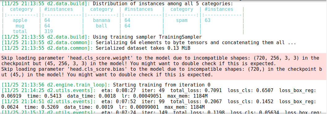
You will see some results printed out, but the default Detectron2 trainer also hooks into TensorBoard for more detailed visualization (even though this is a TensorFlow based product it works with PyTorch as well). To do this,
- Open a Terminal and type
tensorboard --logdir=path/to/training/results
(where this path is dictated bycfg.OUTPUT_DIR) - In your favorite browser, start Tensorboard
(typicallyhttp://localhost:6006/)
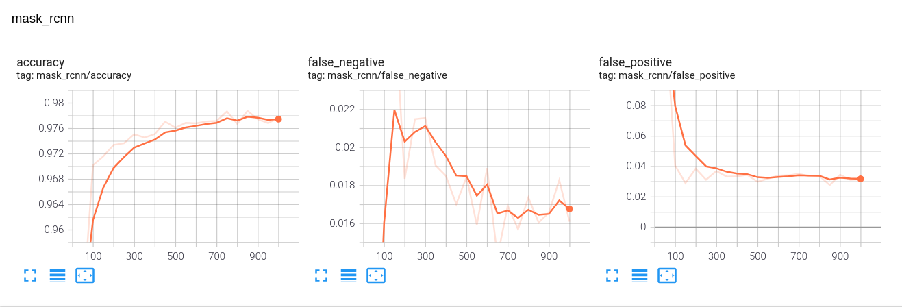
The x-axis is number of iterations (I’m using a batch size of 1 because laptop GPUs)
Analyzing Results and Using the Model for Inference
When training is complete, the trained model weights (along with any checkpoint weights you may have specified) will be saved in the prescribed output folder for you to load later… or right away!
However, any good machine learning workflow will have a separate test set on which to evaluate our network. This is because we should make sure we’re not overfitting to our training data. We can do this directly with the dataset evaluators in Detectron2. Since we are using the COCO format, our evaluation looks like this.
from detectron2.evaluation import COCOEvaluator

# Load weights from the most recent training run
cfg.MODEL.WEIGHTS = os.path.join(cfg.OUTPUT_DIR, "model_final.pth")

# Evaluate on the test set
evaluator = COCOEvaluator(test_dataset_name,
  tasks=("segm",), # Use ("bbox",) for RetinaNet
  distributed=False,
  output_dir="maskrcnn_test_output")
trainer.test(cfg, trainer.model, evaluators=evaluator)
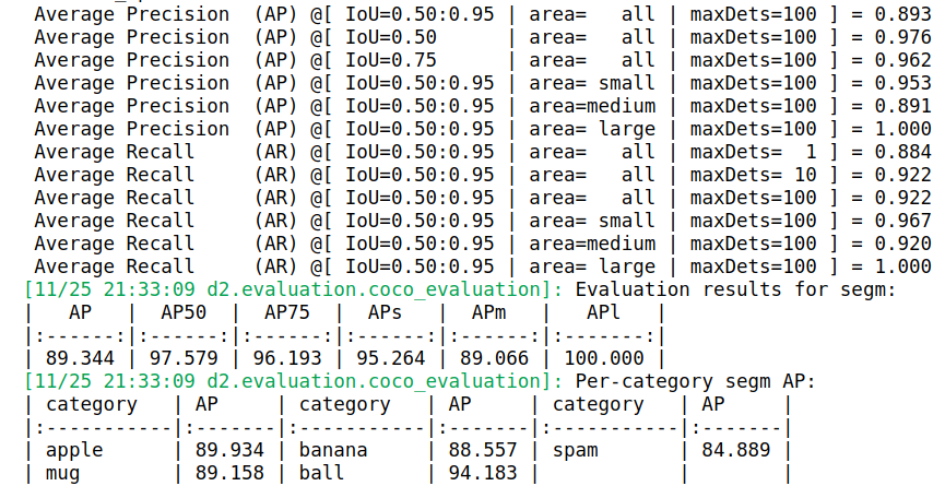
The key metrics in the printout above are:
- Intersection over Union (IoU): Dictates how the ground truth and predicted detections overlap. IoU of 0 means there is no overlap and IoU of 1 means a perfect detection.
- Average Precision (AP): Dictates whether an object detection is deemed correct based on a specified IoU threshold. So when you see AP50, AP75, etc. these denote average precision with IoU thresholds of 0.5, 0.75, etc. And these are often averaged across categories to provide a metric known as mean average precision, or mAP. Again, we want 100% AP but that is quite hard to reach, as our results indicate.
For more detail on object detection metrics, there is a very nice blog post by Jonathan Hui.
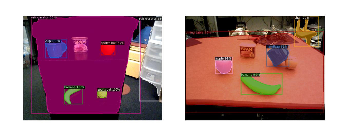
The last thing we need to do is use our network for inference. The code below will use our trained weights and a score threshold of our choice to run the detector on some test images and visualize the results.
# Load weights from the most recent training run
cfg.MODEL.WEIGHTS = os.path.join(cfg.OUTPUT_DIR, "model_final.pth")

# Change the prediction score threshold to a bigger value (e.g. 75%)
cfg.MODEL.ROI_HEADS.SCORE_THRESH_TEST = 0.75

# Create a predictor using the trained model
from detectron2.engine import DefaultPredictor
predictor = DefaultPredictor(cfg)

# Show some qualitative results by predicting on test set images
NUM_TEST_SAMPLES = 5
samples = random.sample(test_dict, NUM_TEST_SAMPLES)
for i, sample in enumerate(samples):
    img = cv2.imread(sample["file_name"])
    outputs = predictor(img)
    visualizer = Visualizer(img, metadata=test_metadata)
    visualizer = visualizer.draw_instance_predictions(
        outputs["instances"].to("cpu"))
    display_img = visualizer.get_image()[:, :, ::-1]
    plt.figure(1+i), plt.xticks([]), plt.yticks([])
    plt.imshow(display_img)

Closing Remarks
I showed how Detectron2 made many things convenient for me. Detectron2 exposes default Python classes for data loading and augmentation, training, evaluating, and more, with some user-tunable parameters. For customization, you can subclass from the same base classes their defaults are derived from, and tack on your own implementations and parameters as needed. However, be ready for a learning curve (as with any other software tool, really). Hopefully this tutorial helps you get started!
It’s also worth reiterating that you can follow these same workflows with the plain “Big 2” machine learning frameworks, which both let you access standard network architectures and pretrained weights. Specifically, PyTorch has torchvision and TensorFlow has TensorFlow Hub.
For the example in this post, check out the code on GitHub, try it for yourself, and contact me if you have any feedback or questions.
One thought on “Object Detection and Instance Segmentation with Detectron2”
Comments are closed.