Introduction to Deep Reinforcement Learning

In the previous post, we introduced reinforcement learning and discussed the classic tabular methods for training agents in environments with finite numbers of discrete states and actions.

The thing is, most practical environments are not tabular, so we can’t represent value functions and/or policies as lookup tables. One approach is to discretize the states and actions of an environment into “bins”, but that has its clear limitations beyond basic examples like the academic pendulum on a cart.

In this post, we will discuss how deep neural networks as function approximators have changed the game in RL over the last decade. This revolution has given rise to many new algorithms that can solve more complex environments with large, or even continuous, state and action spaces. This is what the hype train refers to as deep reinforcement learning.

---

Too Many States: Neural Networks for Value-Based Methods

Suppose we want to train an agent using RL to play a videogame directly from pixels on the screen. While the possible combinations of pixel colors is finite, the number of states is so large that it would be impractical to use a tabular method. Or for a robotics task, suppose your state consists of the joint angles of the robot. These states probably have upper and lower bounds, but they can take any continuous value within that range. Tabular methods won’t work here either.

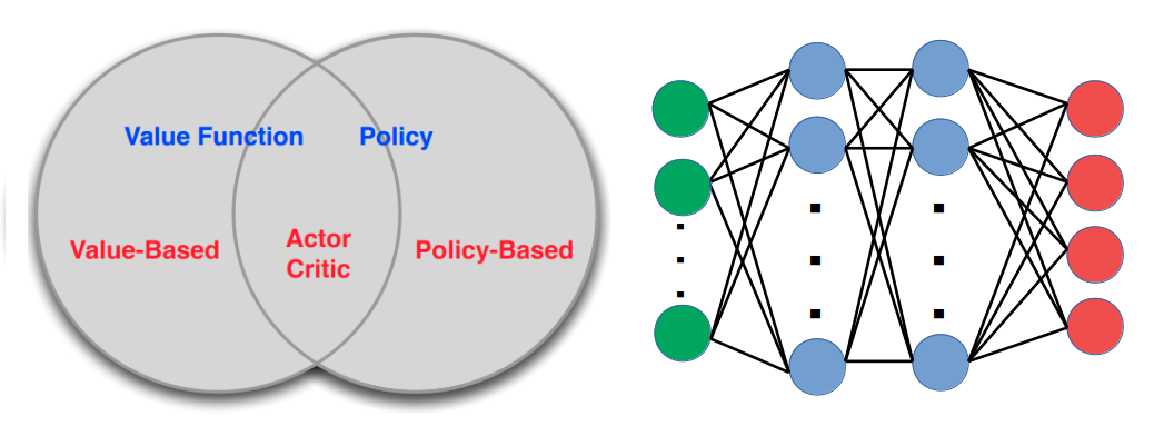
If the action space still consists of a finite set of discrete actions (like up, down, left, right), we can still apply value-based methods… except instead of a value table, we now apply a function approximator that accepts state and outputs an estimated value function for each possible action.

When this function approximator is differentiable (like a linear, polynomial, or exponential function), it means that we can optimize its parameters using gradient-based methods. If our function parameters are given by \(\theta \), our state-value (or Q-value) estimate is then a function \(Q(s,a;\theta)\).

This gave rise to the popular RL method called Deep Q-Learning (DQN) by Mnih et al. in 2013. DQN was shown to learn Atari games by directly mapping from the screen pixels to the joystick actions. As its name suggests, DQN is an adaptation of Q-Learning which uses a deep neural network instead of a table to express its value estimates.

What makes neural networks specifically powerful for RL applications is their:

• High representational capacity as deep chains of piecewise linear functions.
• Ability to encode complex data such as images (e.g., with convolutional neural networks) or temporal sequences (e.g., with recurrent neural networks).

To formalize DQN with some math, recall that Q-Learning used temporal differencing (TD) to define the error term for updating the Q-table… except now it’s not a table, but a neural network. We can define an error — or loss — function that similarly uses TD. For an iteration i, the loss is defined as:

\(L_i(\theta_i) = \mathbb{E} [(y_i – Q(s,a;\theta_i))^2] \)

where \(y_i = r + \gamma \max\limits_{a’} Q(s’,a’;\theta_{i-1}) \) is known as the target. This loss function is the difference between the Q-value estimate at a particular state s and the reward plus discounted value estimate after taking action a and transitioning to the next state s’.

The key difference is that we now have to optimize the neural network parameters using gradient descent which requires us to take the derivative of the loss function with respect to \(\theta_i \) and then apply backpropagation to get the gradient of the neural network itself. This looks like:

\(\nabla_{\theta_i} L_i(\theta_i) = \mathbb{E} [(r + \gamma \max\limits_{a’} Q(s’,a’;\theta_{i-1}) – Q(s,a;\theta_i)) \nabla_{\theta_i} Q(s,a;\theta_i)] \)

Since DQN is also a value-based method, meaning the network provides a Q-value estimate for each action, the policy behaves exactly the same as with Q-Learning. Namely, actions can be selected using a greedy policy that picks the action with the maximum value. In practice we use an ε-greedy policy to ensure the agent explores while learning.

As with many neural network based software frameworks, DQN allows us to collect an experience buffer and randomly sample from that buffer to train the neural network in mini-batches. This is generally true for any deep RL method that is off-policy — meaning, it can use experiences gathered using outdated versions of the policy.

There have been many tweaks to DQN to make it work better. This culminated with an approach by Google DeepMind named Rainbow, which draws parallels from the colors of the rainbow and crams together 6 popular extensions to DQN to show a significant improvement in learning results.

---

Too Many Actions: Policy Gradient Methods

In value-based methods like DQN, we showed how a function approximator that can estimate the value of a specific state-action pair. The policy is to evaluate this function at the current state and take the action that is estimated to have the highest value. This “max” operator is fine when the action space is relatively small, but with a large number of actions this is impractical — and for a continuous action space, this is very difficult (if not impossible) to compute.

Luckily, there is an entire field of policy-based methods at our disposal. Instead of approximating a value function with a parameterized representation (can I just say neural network by now?), we will parameterize the policy itself, \(\pi_{\theta}(a|s)\), in terms of learnable parameters \(\theta \).

• For a discrete-action policy, we typically use a neural network with a softmax output layer.
• For a continuous-action policy, we typically use a neural network that outputs the parameters of a Gaussian distribution (mean and covariance).

What makes this all work is the policy gradient theorem. To explain it simply, recall that we first have to define an objective function — or loss — to optimize over. In this case, the loss function will simply be the value of the initial state s₀, which we want to maximize.

\(J(\theta) = V_{\pi_{\theta}}(s_0) \)

Easy, right? … well, not really, because the value of the initial state is an expectation that depends on the initial state, the state transition dynamics under the policy, and the values of every state that could probably be reached. After a lot of math, whose proof you can find in the Policy Gradient chapter of the Sutton and Barto book, we can get an expression for the gradient of this loss function that only involves the gradient of the policy.

\(\nabla_{\theta}J(\theta) = \mathbb{E}[ Q(s,a) \nabla_{\theta} \log \pi_{\theta}(a|s) ] \)

What makes policy-based methods so diverse is that the use of \(Q(s,a) \) in the above formulation is not mandatory. You can optimize over other quantities that depend on state and/or action. Also, the value can either be estimated purely by sampling them from experience, or even by using another value function approximator (read: neural network). We’ll see a few examples shortly.

One last note before moving on is that there are finite-difference policy gradient methods. This simply means approximating the policy gradient using finite differencing, which saves you a lot of math and headaches up front, but is also way more computationally expensive than having a closed-form gradient to evaluate. In practice, it’s much more common to represent a policy with a differentiable function.

Monte-Carlo Policy Gradient (REINFORCE)

We already discussed Monte-Carlo methods in the previous post, in which we roll out a policy for a few episodes, collect the returns \(G_t \) , and use those returns to get better estimates of our value function. You can similarly apply these methods to policy gradient to get the REINFORCE algorithm.

\(\nabla_{\theta}J(\theta) = \mathbb{E}[ G_t \nabla_{\theta} \log \pi_{\theta}(a|s) ] \)

REINFORCE involves repeating the following method for several episodes.

1. Run an entire episode using the policy \(\pi_{\theta} \).
2. Collect the entire experience \((s_t, a_t, r_{t+1}, s_{t+1}, …) \), which allows you to compute the returns \(G_t \) at every time step t.
3. For each time t in the episode, run a gradient ascent update using the policy gradient \(\theta \leftarrow \theta + \alpha G_t \nabla_{\theta} \log \pi_{\theta}(a|s) \).

As we discussed previously, Monte Carlo methods are unbiased but have high variance. However, there are techniques to reduce variance without affecting bias, such as subtracting a baseline from the return estimates… which gets us into the next section.

---

Best of Both Worlds: Actor-Critic Methods

Going back to the policy gradient theorem, the gradient of our loss function depends on the policy gradient itself as well as a value function. So what if this value was approximated with a separate function?

This is where actor-critic methods come in. Specifically,

• The actor \(\pi_{\theta}(a|s) \) accepts a state and outputs an action, and is parameterized by weights \(\theta \).
• The critic \(Q_w(s,a) \) accepts a state and outputs a predicted Q-value, and is parameterized by weights \(w \). Again, this could be a different type of value function depending on the loss you choose.

During training, the actor and critic networks are both updated using some RL algorithm. When it’s time to deploy, only the trained actor is needed; that is, the critic is only used to help train the actor. Below is the training loop for an action-value (or Q-value) actor-critic method.

1. Sample an action from \(\pi_{\theta}(a|s) \) and collect the new state s’ and reward r.
2. Train the critic using the TD error: \(w \leftarrow w + \alpha_w (r + \gamma Q_w(s’,a’) – Q_w(s,a)) \nabla_w Q_w(s,a) \). Note this requires us to evaluate the policy at state s’ to get a’, which is means this method is on-policy.
3. Train the actor using policy gradient: \(\theta \leftarrow \theta + \alpha_{\theta} Q_w(s,a) \nabla_{\theta} \log \pi_{\theta}(a|s) \).

NOTE: In practice, many actor-critic network formulations will use weight sharing for efficiency. You may also see a single neural network which outputs both action and value estimates. These are implementation details, since backpropagation should take care of however you choose to express your networks at training time.

Let’s compare this to REINFORCE, which is a Monte Carlo approach so it is unbiased but high-variance. Using a critic to estimate the value function introduces bias. However, there is a compatible function approximation theorem which states that if our critic loss is set up to minimize mean-squared error between the value estimate and the true value, the policy gradient theorem still holds. The proof can be found in the original policy gradient paper.

Advantage-Based Actor-Critic Methods

We mentioned earlier that we can reduce variance by subtracting a baseline from the policy gradient. A common baseline to use is an estimate of the state-value function \(V(s) \), since this measures the expected return of a state under the policy \(\pi_{\theta}(a|s) \).

This leads to actor-critic methods that optimize over the advantage function, which is something we have not yet seen in these posts. Advantage is simply the difference between the state-action value and the state value functions, which we can express in words as “how much better it is to take one particular action over others”.

\(A(s,a) = Q(s,a) – V(s) \)

So now we will be dealing with a policy gradient using an advantage function estimator. This resolves to using the TD error \(\delta \) to train both the actor and critic.

• \(\delta = r + \gamma V_w(s’) – V_w(s) \)
• \(w \leftarrow w + \alpha_w \delta \nabla_w Q_w(s,a) \)
• \(\theta \leftarrow \theta + \alpha_{\theta} \delta \nabla_{\theta} \log \pi_{\theta}(a|s) \)

Two common RL algorithms that use this formulation are Advantage Actor-Critic (A2C) and Asynchronous Advantage Actor-Critic (A3C), both of which are introduced in this 2016 paper by Mnih et al. A3C allows for asynchronous training in multithreaded applications, and A2C does the same in a synchronous manner. Due to this distributed nature, the authors use k-step returns rather than one-step returns, such that they can collect multiple experiences before a training update. The method above still holds, except the k-step TD error is now:

\(\delta = \sum_{i=0}^{k} \gamma^i r_i + \gamma^k V_w(s_{t+k}) – V_w(s_t) \)

There are other actor-critic methods designed for scaling up for distributed computing and the use of an experience replay (which typically requires off-policy methods). Two worth looking into are Actor-Critic with Experience Replay (ACER) and Importance Weighted Actor Learner (IMPALA).

Deep Deterministic Policy Gradient (DDPG)

Another important actor-critic method is Deep Deterministic Policy Gradient (DDPG), which was introduced in the paper Continuous Control with Deep Reinforcement Learning by Lillicrap et al. in 2015.

DDPG uses a critic that learns from a TD loss and an actor that learns using policy gradient, which looks similar to the other actor-critic methods we have seen above. However, DDPG is an off-policy method that can use large experience buffers we can sample in batches for sample-efficient training — just as with DQN.

To ensure training stability, DDPG employs soft updates on both the actor and critic networks. This is done by maintaining separate target networks for training whose parameters slowly lag behind the trained networks. In DDPG, the authors use a coefficient \(\tau \ll 1 \) (typically 0.001 to 0.01) to perform these soft updates, where:

• The actor is \(\mu(s|\theta_{\mu}) \), and its target network is \(\mu'(s|\theta_{\mu’}) \).
• The critic is \(Q(s,a|\theta_{Q}) \), and its target network is \(Q'(s,a|\theta_{Q’}) \).

Also, since DDPG has “deterministic” in its name, exploration cannot be done by sampling the probability distribution of the current policy. The authors add Ornstein-Uhlenbeck (OU) process noise \(\mathcal{N} \) to the actions during training, whose parameters are decayed over time to trade off between exploration and exploitation. Other work has shown that adding noise to the network parameters can also be helpful.

Putting it all together, the DDPG algorithm looks as follows:

---

Trust Region and Proximal Policy Optimization

Another way to modify policy gradient methods to use experiences from old versions of the policy is through a technique known as importance sampling. This weights samples based on — in our case — the difference between the action probability distributions given by the current and old policies.

Trust Region Policy Optimization (TRPO) is one such policy gradient method that uses trust region optimization methods to minimize an objective function based on the advantage estimate \(\hat{A}_t \) and the difference in old vs. current policies — all while keeping the KL divergence \(D_{\text{KL}} \) between these policies constrained to a parameter \(\delta \) to prevent drastic changes in the policies.

maximize \(J(\theta) = \mathbb{E} [ \frac{\pi_{\theta}(a|s)}{\pi_{\theta_{\text{old}}}(a|s)} A_{\theta_{\text{old}}}(s,a) ] \)

subject to \(D_{\text{KL}} [ \pi_{\theta_{\text{old}}}(\cdot|s) || \pi_{\theta}(\cdot|s) ) ] \leq \delta \)

Because of how complex TRPO is, and some challenges in allowing fancier flavors of neural network approximators and optimization techniques, OpenAI later came up with a simplified and highly effective version named Proximal Policy Optimization (PPO). PPO does away with the trust-region methods and KL divergence constraint by introducing a clipped surrogate objective that prevents the difference between old and new policy probability ratios from exceeding some parameter ε.

If we define \(r_t(\theta) = \frac{\pi_{\theta}(a_t|s_t)}{\pi_{\theta_{\text{old}}}(a_t|s_t)} \) to make the equations look somewhat less horrifying, then the TRPO and PPO cost functions are shown below.

• TRPO: \(J(\theta) = \mathbb{E} [ r_t(\theta) \hat{A}_t ] \)
• PPO: \(J(\theta) = \mathbb{E} [ \min( r_t(\theta) \hat{A}_t , \text{clip}(r_t(\theta), 1-\epsilon, 1+\epsilon) \hat{A}_t ] \)

The PPO paper also presents an alternative penalty-based surrogate objective, where the KL divergence is treated as a penalty rather than a constraint in the loss function with hyperparameter \(\beta \).

\(J(\theta) = \mathbb{E} [ r_t(\theta) \hat{A}_t – \beta D_{\text{KL}} [ \pi_{\theta_{\text{old}}}(\cdot|s_t) || \pi_{\theta}(\cdot|s_t) ) ] ] \)

To summarize my understanding of TRPO and PPO:

• They are still on-policy methods, but through importance sampling, we can be more sample efficient by allowing some batching of experiences.
• Using penalties on KL divergence and/or a clipped surrogate objective, TRPO and PPO provide additional training stability over pure off-policy methods like DQN and DDPG.
• PPO is a simplified tweak of TRPO that has empirically shown similar performance despite its simplicity, and has largely displaced TRPO in practice.
• While the advantage estimate often comes from a critic network, you can also use sample-based estimates from a trajectory rollout (à la Monte Carlo / REINFORCE) and run TRPO and PPO with only an actor.

---

Conclusion

I hope you have enjoyed reading and it has helped you navigate the daunting world of reinforcement learning with neural networks. Below is a nice graphic from OpenAI that shows some of the popular deep RL algorithms in a similar taxonomy to what we presented in the previous post.

Let’s also revisit the importance of the policy gradient theorem, which spawned an entire camp of deep RL algorithms that can work for high-dimensional and continuous action spaces. Most notably, we saw several actor-critic methods which combine value function approximation with policy gradient.

As discussed in the Policy Gradient lecture of David Silver’s RL course, policy-based methods have advantages and disadvantages compared to value-based methods.

• Can work with high-dimensional or continuous action spaces! (BIG WIN)
• Can learn stochastic policies that are more elaborate than ε-greedy.
• Typically have better convergence properties, but converge to a local rather than a global minimum.
• Evaluating a policy during learning can be inefficient and high-variance.

For an awesome and way more mathematical overview of policy gradient algorithms, which even includes a derivation of the policy gradient theorem, check out Lilian Weng’s blog post.

Finally, let me say it again: Just because these approaches use neural networks doesn’t mean you need to. Any differentiable function with a gradient will work using the methods we discussed in this post. Depending on your problem, a simple function (linear, polynomial, exponential, etc.) may suffice; and if it does, it will be way more computationally efficient than a giant neural network. Or you could even choose to approximate the gradient using finite differencing, though that wouldn’t be my first recommendation without a good reason.

In the next post, I will go into some special topics in RL that did not quite belong here but I nonetheless found interesting. Or if you don’t want to get too researchy, I will also be sharing some useful learning resources to get started with RL. See you then!