An Intuitive Guide to Reinforcement Learning

In this post I will give an overview of reinforcement learning that tries to keep the math to a minimum. Be warned, though, that machine learning algorithms are essentially all math so it’s difficult to do away with notation and equations altogether. Don’t worry — I’ve done my best to explain all the math in words.

As is becoming a common theme with my survey posts, I will start by discussing reinforcement learning before deep learning happened. In the next post, I will move into today’s state of the art which is unsurprisingly full of neural networks. Hope you enjoy!

---

What is Reinforcement Learning?

Reinforcement Learning (RL) is a category of machine learning, alongside supervised and unsupervised learning. Typically, supervised and unsupervised learning algorithms fit a model to an existing set of data (labeled or unlabeled, respectively). RL instead seeks to train a model by having an agent interact with an environment and collecting a numeric reward that indicates how “well” the agent is performing.

So, RL is all about maximizing cumulative reward over time by trial and error. In a way, the reward can be seen as the label for a supervised learning algorithm; however, the fact that reward is collected over time adds some nuance to that gross simplification.

At any given time, the agent will exist in a state \(s_t \) and take an action \(a_t \) which puts it at a new state \(s_{t+1} \) and yields a reward \(r_{t+1} \).

By the way, in the literature you will often see “state” and “observation” (with the variable o) used somewhat interchangeably. The idea is that an agent observes the environment, but this measurement could be perfect or noisy, as well as encompass only a subset of the true state if the environment is partially observable rather than fully observable. Technically, state and observation are equivalent if the environment is fully observable and the observation has no noise.

There are a few more mathematical concepts that you should know, which will come up in the equations throughout the post, and more generally in the RL literature.

• Policy \(\pi (a|s) \) : The policy is the part of the agent that picks an action given a state, and is what we deploy to our environment when training is done.
• Return \(G_t = R_{t+1} + \gamma R_{t+2} + \gamma^2 R_{t+3} + … \) is the cumulative reward from a given state, discounted by a factor \(\gamma \) between 0 and 1 which encodes the agent’s preference towards immediate vs. long-term reward. In practice, this value is usually betwen 0.9 and 0.999 (but never actually 1 for numerical stability reasons over infinite time sequences).
• Value function \(V_{\pi}(s) = \mathbb{E} [G_t | S_t = s] \) is the expected return of following your policy given a starting state.
• State-action value function \(Q_{\pi}(s, a) = \mathbb{E} [G_t | S_t = s, A_t = a] \) is the expected return of given a starting state and action. Because of the long name, typically you’ll hear this being called the “Q-value” or “Q-function”.

The cool thing about the value functions above is that their relationship is recursive, which allows us to use them for learning. This is all a consequence of RL treating environments as a Markov Decision Process (MDPs) where a state transition to a state s’ depends only on the current state s and action a, with probability \(P^a_{ss’} \). The relationships below are derived from the famous Bellman equations.

\(V_{\pi}(s) = \sum\limits_{a} \pi(a|s) \sum\limits_{s’} P^a_{ss’} [R^a_{ss’} + \gamma V_{\pi}(s’)] \)

\(Q_{\pi}(s,a) = \sum\limits_{s’} P^a_{ss’} [R^a_{ss’} + \gamma \sum\limits_{a’} \pi(a’|s’)Q_{\pi}(s’,a’)] \)

---

Taxonomy of RL algorithms

RL algorithms can be classified along many dimensions. You will frequently see the highlighted terms in this section in the RL community, so let’s talk about them before we drill down into some of the actual learning algorithms and return to a little more math.

Model-based vs. model-free:

• In model-based RL, an agent will learn a model (specifically, the state transition function given a state and action) to use with a planning algorithm like Model Predictive Control to maximize return.
• Model-free RL instead directly learns a value function and/or policy based purely on experiences (states, actions, and rewards).

For the rest of this post, we will be exploring model-free RL methods, which can be further categorized.

Discrete vs. continuous states/actions: This isn’t so much a categorization, but something that affects which algorithms you can use depending on your environment. If the environment consists of a finite set of discrete states and actions, then you can apply tabular methods — essentially, you create a lookup table of value functions and pick actions based on the table. A more complex system with a continuous range of observations and actions requires different methods — for example, you can’t use a purely value-based approach if your action space is continuous. If this doesn’t make sense, the next few sections should clear that up!

Value-based vs. policy-based: In value-based methods the agent learns the value of being in a state and taking a specific action. The policy then becomes a choice of which action maximizes return given our estimates of value. In policy-based methods, you are directly learning the policy without explicitly learning the value. Policy-based methods are a little less transparent for this reason, but can cover a wider range of environments. It’s also worth noting that actor-critic methods combine the best of both these models.

On-policy vs. off-policy: Is the agent updating the policy as it explores, thereby always taking actions from the latest policy? Or is it able to continue learning from experiences it took in the past when the policy was vastly different? There are tradeoffs, namely that on-policy methods can be more stable but once you collect an experience and learn from it you must throw it away; for off-policy, you can gather an entire buffer of past experiences and continue using them throughout learning. We therefore say that off-policy methods tend to be more sample efficient.

---

Tabular Methods: Discrete State, Discrete Action Systems

Let’s start with one of the well-known academic environments for reinforcement learning: the grid world.

This grid world has the following properties.

• States: Each grid cell is a separate state
• Actions: At each cell, you can take one of 4 actions — left, right, up, or down. These actions could be deterministic (we know exactly which state we transition to) or stochastic (there are nonzero probabilities on ending in another state).
• Reward: The agent gets a negative reward every time it does not visit a terminal state. In other words, the incentive is to reach a terminal state to maximize reward — in this case, to stop collecting negative reward as quickly as possible.

These types of systems with finite numbers of discrete states and actions were the first to be explored and solved with reinforcement learning. We refer to these approaches as tabular methods, since the value functions and policies can be represented as tables that depend on the state and/or actions.

What if the Environment is Known?

If the environment model is fully known, we can apply exhaustive search — that is, search for all possible outcomes. For simple tasks like playing a game of tic-tac-toe, this is easy to achieve. However, search complexity grows exponentially in the number of states and actions, so it’s not very practical for most interesting problems we want to solve.

Another set of methods is dynamic programming, which allows us to iteratively solve for an optimal policy without exhaustive search, but rather by looking at state transitions one at a time. The two main approaches used in RL are known as policy iteration and value iteration.

In the examples below, we will show these approaches for our grid world, assuming for simplicity that the actions are fully deterministic and using a discount factor \(\gamma = 1 \).

Policy Iteration

First, we start with an initial policy \(\pi \), which is usually random. Then, policy iteration involves an alternating sequence of steps known as policy evaluation and policy improvement.

• Policy evaluation uses the current policy to estimate the value for a state: \(V(s) = \sum\limits_{a} \pi(a|s) \sum\limits_{s’} P^a_{ss’} [R^a_{s} + \gamma V_{\pi}(s’)] \).
• Policy improvement then takes these updated value estimates and updates the policy by greedily choosing the action that will take the agent to the highest-value state. If there are multiple, choose one randomly.

We say that policy iteration has converged when the policy improvement step does not change the previous policy. Keep in mind that it is not necessary to wait for value estimates from policy evaluation under a particular policy to converge before moving to policy improvement, as this would be inefficient. In practice, a policy iteration loop will alternate between a few steps of policy iteration and then one step of policy improvement.

Value Iteration

In principle, this is quite similar to policy iteration, but here we iterate only through estimates of the states’ value functions until those estimates converge. It is not until the end of these iterations that we look at the policy.

We start with an initial guess for the value function at each state — for example, all zeros. We can then iteratively calculate the value function of that state from our estimates by finding the maximum (discounted) value over all adjacent states, plus the reward of moving to that state. Updating the value estimate from an iteration k to a new iteration k+1 looks like this for each state s:

\(V_{k+1}(s) \leftarrow \max\limits_{a} \sum\limits_{s’} P^a_{ss’} [R^a_{s} + \gamma V_{k}(s’)] \)

This is guaranteed to converge to the true values of the states given infinite iterations, but in practice we often stop when the value estimates stop changing past a given threshold — similar to policy evaluation, but here this is done only once.

The policy is then backed out of the final value estimates by picking value functions greedily, as is done in policy improvement; except that in value iteration, we only do this once at the end.

Learning Without a Model

While search and dynamic programming converge to an optimal solution, they require us to know the full environment model and its reward structure. If we don’t have this, we get into the camp of model-free reinforcement learning in which we are purely learning a policy by interacting with an unknown environment.

The two main approaches for model-free RL are Monte Carlo and Temporal Differencing (TD) methods. The biggest differences are:

• Monte Carlo methods will roll out a policy for an entire episode — that is, until a terminal state is reached — and the math deals with the final return value.
• TD methods will look at the difference in the estimated return vs. the actual observed return over a specified time interval.

With TD methods, you will often see a number attached to them — for example, TD(0) or TD(1). Generally, these all belong to a general family of methods called TD(λ), where λ can range between 0 and 1.

• TD(0) means that we only look one time step ahead.
• TD(1) is equivalent to Monte Carlo — meaning we look at the return at the end of the episode.
• Any TD(λ) for λ between 0 and 1 is a weighted sum of the above — that is, we partially consider returns one time step ahead, two time steps ahead, and so on until we observe the full trajectory.

What, then, is the tradeoff between TD(0) and Monte Carlo / TD(1)?

• Monte Carlo has high variance, TD has low variance. This comes from the fact that Monte Carlo estimates the value of a state-action pair from a rollout of many actions over the entire episode, whereas the TD update rule uses one step.
• Monte Carlo has zero bias, TD has some bias. Monte Carlo methods consider consider a full episode to estimate value, so there is no bias in that estimate. On the other hand, TD introduces bias from the initial choice of value estimates.

---

Aside: Exploration vs. Exploitation

With these RL algorithms, it can be easy to get stuck in a bad local minimum. Suppose you start with an estimate that every state-action pair has a value of 0. As soon as you take an action that yields positive reward, a learning algorithm following a greedy policy will simply continue to take that action over and over without ever breaking out. This is obviously not good.

This leads to an important concept in RL of the tradeoff between exploitation and exploration.

• Exploitation means acting greedily, i.e., taking the action that you believe will yield the highest return
• Exploration means acting stochastically, i.e., intentionally taking a seemingly “bad” action with the hopes that you discover a better solution.

For any agent that chooses from a finite set of discrete actions, the de facto strategy is to use an ε-greedy (epsilon-greedy) policy, where ε is the probability between 0 and 1 that you take a random action instead of the greedy action that yields the best estimated value. Typically, learning algorithms will start with a high value of ε at the start and then decay down to a small (but nonzero) value at the end. Then, common practice is to deploy a fully greedy policy after the model has been fully trained.

---

Monte Carlo Learning Methods

Monte Carlo methods involve running lots and lots of simulations and relying on the law of large numbers in the hopes that all the samples we collected represent the true probabilistic distribution.

In RL, this is no different. We run several episodes of an agent executing a policy in an environment, and the returns we observe for each of these episodes hopefully provides us with value function estimates that can guide us towards a better policy. The general method looks something like this:

1. Run an entire episode using some policy.
2. Collect the entire experience \((S_t, A_t, R_{t+1}, S_{t+1}, …) \), which allows you to compute the returns for every state.
3. To learn the state-action values (or Q-values) for each state, take the average of all the Q-values you have ever seen so far for that state-action pair. Statistically speaking, if you run infinite simulations and explore each state infinitely many times, this should converge to the true value of that state.
4. Use the new Q-value estimates to update the policy, ensuring it is ε-greedy because exploration is important.

Mathematically, the update rule will look as follows for each state-action pair \({S_t, A_t} \) observed during an episode:

• Calculate the return for the state-action pair \(G_t = R_{t+1} + \gamma R_{t+2} + \gamma^2 R_{t+3} + … \)
• Update the number of times you have seen that particular state-action pair: \(N(S_t, A_t) \leftarrow N(S_t, A_t) + 1 \)
• Update the estimate of the Q-value of that pair by incorporating this latest return: \(Q(S_t, A_t) \leftarrow Q(S_t, A_t) + \frac{1}{N(S_t, A_t)}(G_t – Q(S_t, A_t)) \)

Note: There are actually two types of Monte Carlo methods knows as first-visit and every-visit. First-visit means we only consider the first instance of that state-action pair in an episode to estimate our value functions, whereas every-visit considers … every visit. First-visit Monte Carlo gives us less data points since we have to throw some away, but it provides a truly unbiased estimate whereas every-visit Monte Carlo adds some bias. Yet another design tradeoff to consider.

---

Temporal Difference Learning Methods

Two of the most common learning algorithms based on TD are SARSA^† and Q-Learning. They both use a very similar update rule, with the exception that SARSA is on-policy and Q-Learning is off-policy.

SARSA:

\(Q(s,a) \leftarrow Q(s,a) + \alpha [R + \gamma Q(s’,a’) – Q(s,a)] \)

To express this in words, the state-action value \(Q(s,a) \) is updated by experience using a learning rate ⍺ which you can tune. This error is the temporal difference between the state-value estimate for the current state before taking an action \(Q(s,a) \) and after taking an action \(R + \gamma Q(s’,a’) \) (the reward from changing states plus the next discounted state-action value estimate). If these two quantities happen to be the same, then the error is zero which means the value estimate has converged for that state-action pair.

^†In case you were wondering, SARSA stands for “state-action-reward-state-action”.

Q-Learning:

\(Q(s,a) \leftarrow Q(s,a) + \alpha [R + \gamma \max\limits_{a’} Q(s’,a’) – Q(s,a)] \)

Notice the only difference with SARSA is that “max” operator in the Q-value estimate after taking the transition. This is necessary because Q-Learning is an off-policy method, so it could use experiences sampled from an outdated version of the policy. Therefore, our estimate of Q (specifically, the a’ term) cannot come directly from the policy but rather by taking a new greedy estimate given the latest Q-values during training.

Q-Learning is arguably the most popular RL algorithm from the repertoire of traditional (pre-deep learning) methods. In fact, it directly gave rise to the first method that demonstrated RL with neural networks, but we’ll save that for the next post.

---

Conclusion

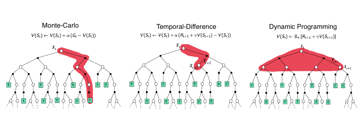
To summarize, let’s compare the backup diagrams in the diagram below.

• Exhaustive search and dynamic programming methods use full knowledge of the environment model and reward structure to explore every possible state-action-reward combination. Thus, it is guaranteed to converge to an optimal solution.
• Monte Carlo and Temporal Difference methods, on the other hand, collect experience by interacting with the environment without knowing an explicit model. MC uses an entire trace up to a terminal state whereas TD methods only consider single transitions.

So how do we choose between a Monte Carlo vs. a TD approach to solve our problem?

• Trading off between bias and variance. As we saw previously, Monte Carlo methods have zero bias and high variance, whereas TD methods have low variance and some bias. However, recall that we could employ TD(λ) methods to be somewhere between these extremes.
• Monte Carlo only works on episodic tasks since learning has to happen over an entire sequence that yields a final return. TD, on the other hand, can learn from incomplete sequences which makes it work for continuous tasks.
• TD can learn online. Unlike Monte Carlo methods, TD methods do not need to wait until an episode is complete to calculate the final return.

Another cool diagram from David Silver’s course is the unified view of RL algorithms below, which succinctly summarizes everything we have discussed in this post.

See you all in the next post, which will build on this background to discuss some of the state-of-the art approaches in the realm of deep reinforcement learning. Stay tuned!