In the previous post, we introduced task planning in robotics. This field broadly involves a set of planning techniques that are domain-independent: That is, we can design a domain which describes the world at some (typically high) level of abstraction, using some modeling language like PDDL. However, the planning algorithms themselves can be applied to any domain that can be modeled in that language, and critically, to solve any valid problem specification within that domain.
The key takeaway of the last post was that task planning is ultimately search. These search problems are often challenging and grow exponentially with the size of the problem, so it is no surprise that task planning is often symbolic: There are relatively few possible actions to choose from, with a relatively small set of finite parameters. Otherwise, search is prohibitively expensive even in the face of clever algorithms and heuristics.
Bridging the gap between this abstract planning space and the real world, which we deeply care about in robotics, is hard. In our example of a mobile robot navigating a household environment, this might look as follows: Given that we know two rooms are connected, a plan that takes our robot from room A to room B is guaranteed to execute successfully. Of course, this is not necessarily true. We might come up with a perfectly valid abstract plan, but then fail to generate a dynamically feasible motion plan through a narrow hallway, or fail to execute a perfectly valid motion plan on our real robot hardware.
This is where Task and Motion Planning (TAMP) comes in. What if our planner spends more effort deliberating about more concrete aspects of a plan before executing it? This presents a key tradeoff in more up-front computation, but a lower risk of failing at runtime. In this post we will explore a few things that differentiate TAMP from “plain” task planning, and dive into some detailed examples with the pyrobosim and PDDLStream software tools.
Some Motivating Examples
Before we formalize TAMP further, let’s consider some tricky examples you might encounter with purely symbolic planning in robotics applications.
In this first example, our goal is to pick up an apple. In purely symbolic planning where all actions have the same cost, there is no difference in navigating to table0 and table1, both of which have apples. However, you will notice that table0 is in an unreachable location. Furthermore, if we decide to embed navigation actions with a heuristic cost such as straight-line distance from the starting point, our heuristic below will prefer table0 because it’s closer to the robot’s starting position than table1.
It wouldn’t be until we try to refine our plan — for example, using a motion planner to search for a valid path to table0 in the unreachable room — that we would fail, have to update our planning domain to somehow flag that main_room and unreachable are disconnected, and then replan with this new information.
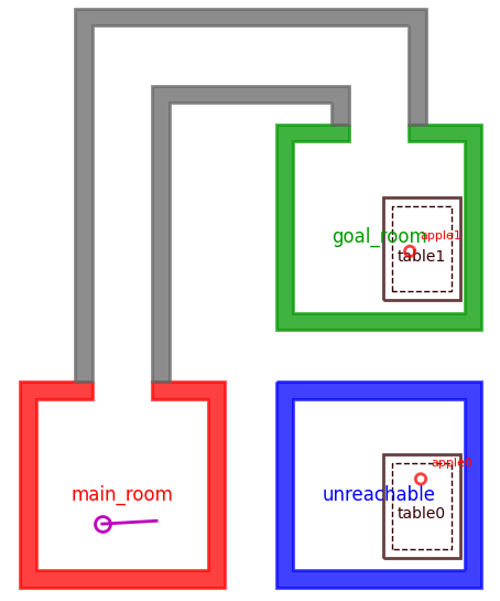
Both
table0 and table1 can lead to solving the goal specification of holding an apple, but table0 is completely unreachable.In this second example, we want to place a banana on a desk. As with the previous example, we could choose to place this object on either desk0 or desk1. However, in the absence of more information — and especially if we continue to treat nearby locations as lower cost — we may plan to place banana0 on desk0 and fail to execute at runtime because of the other obstacles.
Here, some alternative solutions would include placing banana0 on desk1, or moving one of the other objects (water0 or water1) out of the way to enable banana0 to fit on desk0. Either way, we need some notion of collision checking to enable our planner to eliminate the seemingly optimal, but in practice infeasible, plan of simply placing the object on desk0.
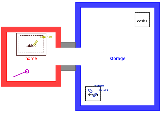
Placing
banana0 on either desk0 or desk1 will satisfy the goal, but desk0 has other objects that would lead to collisions. So, banana0 must either placed on desk1, or the objects need to be rearranged and/or moved elsewhere to allow banana0 to fit on desk0.In both cases, what we’re missing from our purely symbolic task planner is the ability to consider the feasibility of abstract actions before spitting out a plan and hoping for the best. Specifically for embodied agents such as robots, which move in the physical world, symbolic plans need to be made concrete through motion planning. As seen in these two examples, what if our task planner also required the existence of a specific path to move between two locations, or a specific pose for placing objects in a cluttered space?
What Is Task and Motion Planning?
In our examples, the core issue is that if our task planning domain is too abstract, a seemingly valid plan is likely to fail down the line when we call a completely decoupled motion planner to try execute some portion of that plan. So, task and motion planning is exactly as its name states — jointly thinking about tasks and motion in a single planner. As Garrett et al. put it in their 2020 survey paper, “TAMP actually lies between discrete “high-level” task planning and continuous “low-level” motion planning”.
However, there is no free lunch. When considering all the fine details up front in deliberative planning, search becomes expensive very quickly. In symbolic planning, an action may have a discrete, finite list of possible goals (let’s say somewhere around 5-10), so it may be reasonable to exhaustively search over these and find the one parameter that is optimal according to our model. When we start thinking about detailed motion plans that have a continuous parameter space spanning infinite possible solutions, this becomes intractable. So, several approaches to TAMP will apply sampling-based techniques to make planning work in continuous action spaces.
Another way to ensure TAMP is practical is to leverage hierarchy. One popular technique for breaking down symbolic planning into manageable pieces is Hierarchical Task Networks (HTNs). In these 2012 lecture slides, Nilufer Onder mentions “It would be a waste of time to construct plans from individual operators. Using the built-in hierarchy helps escape from exponential explosion.” An example of hierarchical planning is shown in the diagram below. Using this diagram, you can explore the benefits of hierarchy; for example, this planner would never have to even consider how to open a door if the abstract plan didn’t require going down the hallway.
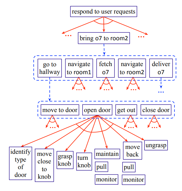
Source: Automated Planning and Acting (2016)
Hierarchical planning is great in that it helps prune infeasible plans before spending time producing detailed, low-level plans. However, in this space the mythical downward refinement property is often cited. To directly quote the 1991 paper by Bacchus and Yang, this property states that “given that a concrete-level solution exists, every abstract solution can be refined to a concrete-level solution without backtracking across abstract levels”. This is not always (and I would argue rarely) achievable in robotics, so backtracking in hierarchical planning is largely unavoidable.
To this end, another strategy behind TAMP has to do with commitment in sampling parameters during search. In the literature, you will see many equivalent words thrown around, but I find the main distinction is between the following strategies:
- Early-commitment (or binding) strategies will sample action parameters from continuous space before search, effectively converting the problem to a purely discrete task planning problem.
- Least-commitment (or optimistic) strategies will instead come up with a purely symbolic plan skeleton. If that skeleton is feasible, then the necessary parameter placeholders are filled by sampling.
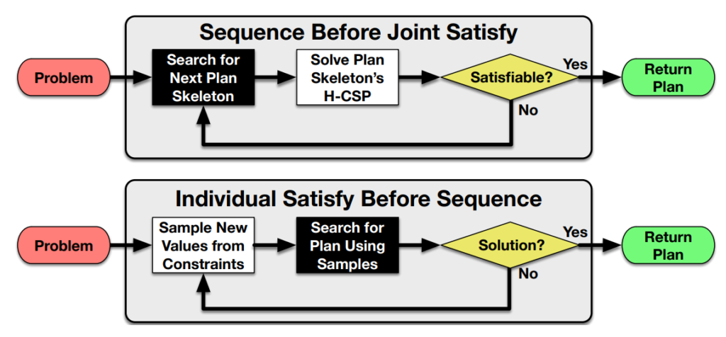
*H-CSP = hybrid constraint satisfaction problem
Source: Garrett et al. (2020), Integrated Task and Motion Planning
Both strategies have advantages and disadvantages, and in practice modern TAMP methods will combine them in some way that works for the types of planning domains and problems being considered. Also, note that in the diagram above both strategies have a loop back to the beginning when a solution is not found; so backtracking remains an unavoidable part of planning.
One key paper that demonstrated the balance of symbolic search and sampling was Sampling-based Motion and Symbolic Action Planner (SMAP) by Plaku and Hager in 2010. Around the same time, in 2011, Leslie Kaelbling and Tomás Lozano-Pérez presented Hierarchical Planning in the Now (HPN), which combined hierarchy and sampling-based techniques for TAMP. However, the authors themselves admitted the sampling part left something to be desired. There is a great quote in this paper which foreshadows some of the other work that would come out of their lab:
Because our domains are infinite, we cannot consider all instantiations of the operations. Our current implementation of suggesters only considers a small number of possible instantiations of the operations. We could recover the relatively weak properties of probabilistic completeness by having the suggesters be generators of an infinite stream of samples, and managing the search as a non-deterministic program over those streams.
Leslie pack kaelbling and Tomás Lozano-Pérez (2011)
hierarchical planning in the now
Directly following this quote is the work their student Caelan Garrett took on — first in the creation of STRIPStream in 2017 and then PDDLStream in 2018. The astute reader will have noticed that PDDLStream is the actual software used in these blog posts, so take this “literature review” with this bias in mind, and keep reading if you want to learn more about TAMP with this specific tool.
If you want to know more about TAMP in general, I will refer you to two recent survey papers that I found useful:
- Integrated Task and Motion Planning, by Garrett et al. (2020)
- Combining task and motion planning: Challenges and Guidelines, by Mansouri et al. (2021)
Mobile Robot Example, Revisited
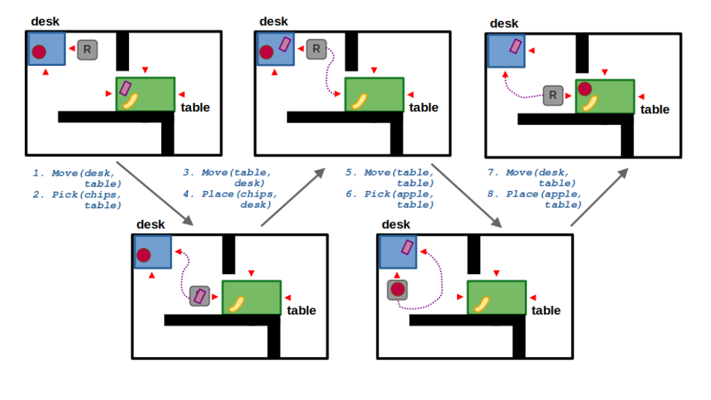
To illustrate the benefits of integrated TAMP, we’ll continue the same mobile robotics example from the previous post. In this problem,
- The robot’s goal is to place the apple on the table.
- Navigation now requires coming up with a goal pose (which is a continuous parameter), as well the actual path from start to goal. For this example, we are using a Rapidly-exploring Random Tree (RRT), but you could swap for any other path-finding algorithm.
- Placing an object now requires sampling a valid pose that is inside the placement surface polygon and does not collide with other objects on that surface.
As you read the following list explaining this problem, make sure you scroll through the slideshow below to get a visual representation.
STEP 1: Looking at the state of the world, you can see how a purely symbolic task planner would output a relatively simple plan: pick the apple, move to the table, and place the apple on the table. In the context of TAMP, this now represents a plan skeleton which several parameters that are yet to be filled — specifically,
?ptis the pose of the robot when navigating to the table?pathis the actual output of our motion planner to get to?pt?pa-1is the new pose of the apple when placed on the table (which follows from its initial pose?pa-0)
STEP 2: To make the problem a little simpler, we made it such that every location has a discrete, finite set of possible navigation locations corresponding to the edges of its polygon. So looking at the table location, you see there are 4 possible navigation poses pt-T, pt-B, pt-L, and pt-R corresponding to the top, bottom, left, and right sides, respectively. Since this set of locations is relatively small, we can sample these parameters up front (or eagerly) at the start of search.
STEP 3: Our move action can now have different instantiations for the goal pose ?pt that are enumerated during search. This is in contrast with the ?path argument, which must be sampled by calling our RRT planner. We don’t want to do this eagerly because the space of paths is continuous, so we prefer to defer sampling of this parameter. If our action has a cost associated with the length of a path, we could imagine that the lowest-cost action would be to navigate to the left side of the table (pt-L), and some randomly sampled path (path42) may describe how we get there.
STEP 4: Next comes the place action, which now must include a valid collision-free pose for the apple on the table. Because of how we set up our problem, our robot cannot find a valid placement pose when approaching from the left side of the table. So, we must backtrack.
STEP 5: After backtracking, we need to find an alternative navigation pose for the table (?pt). Given our environment, the only other feasible location is the bottom side of the table (pt-b), as the walls block the robot from the top and right sides and it would be impossible to find a valid path with our RRT. However, when the robot is at the bottom side of the table, it can also sample a valid placement pose! In our example, the placeholder ?pa-1 is therefore satisfied with some randomly sampled pose pa29.
STEP 6: … And there you have it! A valid plan that defines a sequence of symbolic actions (pick, move, place) along with the necessary navigation pose, path to that pose, and placement location for the apple. It’s not optimal, but it is probabilistically complete!
Now, suppose we change our environment such that we can only approach the table from the left side, so there is no way to directly find a valid placement pose for the apple. Using the same planner, we should eventually converge on a task and motion plan that rearranges the objects world — that is, it requires moving one of the other objects on the table to make room for the apple.
Implementing TAMP with PDDLStream
We will now revisit our pathological examples from the beginning of this post. To do this, we will use PDDLStream for planning and pyrobosim as a simple simulation platform. For quick background on PDDLStream, you may refer to this video.
The key idea behind PDDLStream is that it extends PDDL with a notion of streams (remember the earlier quote from the Hierarchical Planning in the Now paper?). Streams are generic, user-defined Python functions that sample continuous parameters such as a valid sample certifies that stream and provides any necessary predicates that (usually) act as preconditions for actions. Also, PDDLStream has an adaptive technique that balances exploration (searching for discrete task plans) vs. exploitation (sampling to fill in continuous parameters).
Goal-Directed Navigation
We can use PDDLStream to augment our move action such that it includes metric details about the world. As we saw in our illustrative example, we now must factor in the start and goal pose of our robot, as well as a concrete path between those poses.
(:action move
    :parameters (?r ?loc1 ?loc2 ?pose1 ?pose2 ?path)
    :precondition (and (Robot ?r)
                       (Location ?loc1) (Location ?loc2)
                       (Pose ?p1) (Pose ?p2) (Path ?path)
                       (At ?r ?loc1) (AtPose ?r ?pose1)
                       (NavPose ?loc2 ?pose2)
                       (Motion ?pose1 ?pose2 ?path)
    :effect (and (At ?r ?loc2) (not (At ?r ?loc1))
                 (AtPose ?r ?pose2) (not (AtPose ?r ?pose1))
                 (increase (total-cost) (PathLength ?path)))
)
As additional preconditions for this action, we must ensure that:
- The navigation pose is valid given the target location (
NavPose) - There must be a valid path from the start to goal pose (
Motion)
Additionally, we are able to now use more realistic costs for our action by calculating the actual length of our path produced by the RRT! The separate file describing the streams for this action may look as follows. Here, the s-navpose stream certifies the NavPose predicate and the s-motion stream certifies the Motion predicate.
; Samples a pose from a finite set of navigation poses for that location.
(:stream s-navpose
    :inputs (?loc)
    :domain (Location ?loc)
    :outputs (?p)
    :certified (and (Pose ?p) (NavPose ?loc ?p))
)

; Samples a valid path from one pose to another
(:stream s-motion
    :inputs (?p1 ?p2)
    :domain (and (Pose ?p1) (Pose ?p2))
    :outputs (?pth)
    :certified (and (Path ?pth) (Motion ?p1 ?p2 ?pth))
)
The Python implementations for these functions would then look something like this. Notice that the get_nav_poses function returns a finite set of poses, so the output is a simple Python list. On the other hand, sample_motion can continuously spit out paths from our RRT, and it implemented as a generator:
def get_nav_poses(loc):
    """
    Gets a list of navigation poses for a specific location.
    """
    return [(p,) for p in loc.nav_poses]

def sample_motion(planner, p1, p2):
    """
    Samples a motion plan from a start to a goal pose.
    """
    while True:
        path = planner.plan(p1, p2)
        if path is None:
            break
        yield (path,)
Putting this new domain and streams together, we can solve our first pathological example from the introduction. In the plan below, the robot will compute a path to the farther away, but reachable room to pick up an apple and satisfy the goal.
Object Manipulation
Similarly, we can extend our place action to now include the actual poses of objects in the world. Specifically,
- The
?placeposeargument defines the target pose of the object. - The
Placeablepredicate is certified by as-placestream. - The
IsCollisionFreepredicate is actually a derived predicate that checks individual collisions between the target object and all other objects at that location. - Each individual collision check is determined by the
CollisionFreepredicate, which is certified by at-collision-freesteam.
(:action place
    :parameters (?r ?o ?loc ?placepose)
    :precondition (and (Robot ?r) (Object ?o) (Location ?loc)
                       (Pose ?placepose)
                       (At ?r ?loc)
                       (Holding ?r ?o)
                       (Placeable ?loc ?o ?placepose)
                       (IsCollisionFree ?loc ?o ?placepose)
    :effect (and (HandEmpty ?r)
                 (At ?o ?loc) (AtPose ?o ?placepose)
                 (not (Holding ?r ?o))
                 (increase (total-cost)
                     (PlaceCost ?loc ?o ?placepose))
            )
)

(:derived (IsCollisionFree ?loc ?o ?p)
    (not (exists (?obs ?pobs)
                 (and (Obj ?obs) (Pose ?pobs)
                      (At ?obs ?loc) (AtPose ?obs ?pobs)
                      (not (CollisionFree ?o ?p ?obs ?pobs))
                 )
         )
    )
)


; STREAMS (in a separate file)
; Samples an object placement pose.
(:stream s-place
    :inputs (?loc ?o)
    :domain (and (Location ?loc) (Obj ?o))
    :outputs (?p)
    :certified (and (Pose ?p) (Placeable ?loc ?o ?p))
)

; Checks if a placement pose is collision free.
(:stream t-collision-free
    :inputs (?o1 ?p1 ?o2 ?p2)
    :domain (and (Obj ?o1) (Pose ?p1)
                 (Obj ?o2) (Pose ?p2))
    :certified (CollisionFree ?o1 ?p1 ?o2 ?p2)
)
The Python implementation for sampling placement poses and checking for collisions may look as follows. Here, sample_place_pose is our generator for placement poses, whereas test_collision_free is a simple Boolean (true/false) check.
def sample_place_pose(loc, obj, padding=0.0, max_tries=100):
    """
    Samples a placement pose for an object at a location.
    """
    obj_poly = inflate_polygon(obj.raw_polygon, padding)
    while True:
        is_valid_pose = False
        while not is_valid_pose:
            # Sample valid pose from the location polygon.
            pose_sample = sample_from_polygon(
                loc.polygon, max_tries=max_tries)

            # Check that the object is inside the polygon.
            poly_sample = transform_polygon(
                obj_poly, pose_sample)
            is_valid_pose = poly_sample.within(loc.polygon)
            if not is_valid_pose:
                continue  # If sample is in collision, retry.

        yield (pose_sample,)

def test_collision_free(o1, p1, o2, p2, padding=0.0):
    """
    Test for collisions between objects at specified poses.
    """
    o1_poly = transform_polygon(
        inflate_polygon(o1.raw_polygon, padding), p1)
    o2_poly = transform_polygon(o2.raw_polygon, p2)
    return not o1_poly.intersects(o2_poly)
By expanding our domain to reason about the feasibility of object placement, we can similarly solve the second pathological example from the introduction. In the first video, we have an alternative location desk1 where the robot can place the banana and satisfy the goal.
In the second video, we remove the alternative desk1. The same task and motion planner then produces a solution that involves picking up one of the objects on desk0 to make room to later place the banana there.
You can imagine extending this to a more realistic system — that is, one that is not a point robot and has an actual manipulator — that similarly checks the feasibility of a motion plan for picking and placing objects. While it wasn’t the main focus of the work, our Active Learning of Abstract Plan Feasibility work did exactly this with PDDLStream. Specifically, we used RRTs to sample configuration-space paths for a Franka Emika Panda arm and doing collision-checking using a surrogate model in PyBullet!
Conclusion
In this post we introduced the general concept of task and motion planning (TAMP). In theory, it’s great to deliberate more — that is, really think more about the feasibility of plans down to the metric level — but with that comes more planning complexity. However, this can pay off in that it reduces the risk of failing in the middle of executing a plan and having to stop and replan.
We introduced 3 general principles that can make TAMP work in practice:
- Hierarchy, to determine the feasibility of abstract plans before planning at a lower level of refinement.
- Continuous parameter spaces, and techniques like sampling to make this tractable.
- Least-commitment strategies, to come up with symbolic plan skeletons before spending time with expensive sampling of parameters.
We then dug into PDDLStream as one tool for TAMP, which doesn’t do much in the way of hierarchy, but certainly tackles continuous parameter spaces and least-commitment strategies for parameter binding. We went through a few examples using pyrobosim, but you can access the full set of examples in the pyrobosim documentation for TAMP.
The PDDLStream repository has many more examples that you can check out. And, of course, there are many other task and motion planners out there that focus on different things — such as hierarchy without continuous parameters, or factoring in other common objectives such as temporal aspects and resource consumption.
Hope you have enjoyed these posts! If the tools shown here give you any cool ideas, I would love to hear about them, so feel free to reach out.


3 thoughts on “Integrated Task and Motion Planning in Robotics”